Simple, Multiple Linear and Stepwise Regression (with Example)
Linear regression (OLS): theory + practice
Linear regression models the conditional mean of a response as a
linear function of predictors: \(\mathbb{E}[Y
\mid X] = X\beta\).
Under the classical assumptions (linearity in parameters, zero-mean
errors conditional on \(X\),
homoscedasticity, no perfect multicollinearity), OLS is BLUE:
best linear unbiased estimator.
We cover:
- Simple regression (by hand +
lm()). - Multiple regression (diagnostics, collinearity, inference).
- Regression with factors (dummy coding, reference levels).
- Stepwise regression (AIC) + out-of-sample validation.
1) Simple linear regression
Model: \[ y_i = \beta_0 + \beta_1 x_i + \epsilon_i, \quad \mathbb{E}[\epsilon_i \mid x_i] = 0 \]
Data + scatterplot
library(ggplot2)
library(readr)

women_df <- read_csv("raw_data/women.csv", show_col_types = FALSE)

ggplot(women_df, aes(x = height, y = weight)) +
  geom_point(size = 2) +
  geom_smooth(method = "lm", se = TRUE, color = "steelblue") +
  theme_classic() +
  labs(title = "Women dataset: height vs weight")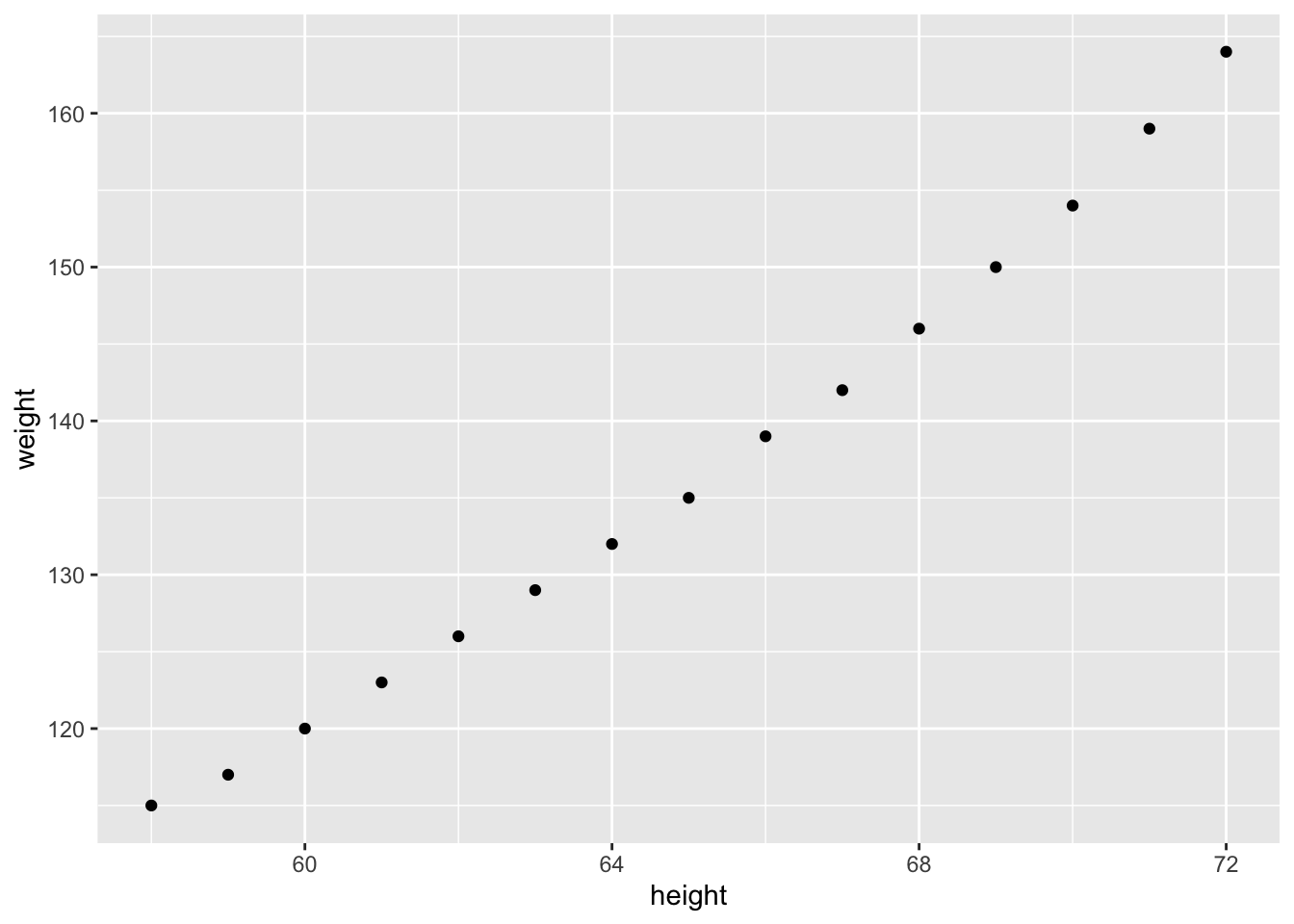
OLS estimates (by hand)
In simple regression: \[ \hat{\beta}_1 = \frac{\text{Cov}(x,y)}{\text{Var}(x)}, \quad \hat{\beta}_0 = \bar{y} - \hat{\beta}_1 \bar{x} \]
beta_1 <- cov(women_df$height, women_df$weight) / var(women_df$height)
beta_0 <- mean(women_df$weight) - beta_1 * mean(women_df$height)
c(beta_0 = beta_0, beta_1 = beta_1)
## beta_0 beta_1
## -87.51667 3.45000Fit with lm() + interpretation
##
## Call:
## lm(formula = weight ~ height, data = women_df)
##
## Residuals:
##     Min      1Q  Median      3Q     Max
## -1.7333 -1.1333 -0.3833  0.7417  3.1167
##
## Coefficients:
##              Estimate Std. Error t value Pr(>|t|)
## (Intercept) -87.51667    5.93694  -14.74 1.71e-09 ***
## height        3.45000    0.09114   37.85 1.09e-14 ***
## ---
## Signif. codes:  0 '***' 0.001 '**' 0.01 '*' 0.05 '.' 0.1 ' ' 1
##
## Residual standard error: 1.525 on 13 degrees of freedom
## Multiple R-squared:  0.991,  Adjusted R-squared:  0.9903
## F-statistic: 1433 on 1 and 13 DF, p-value: 1.091e-14## (Intercept) height
## -87.51667 3.45000Confidence interval vs prediction interval
A confidence interval targets the mean response \(\mathbb{E}[Y \mid X=x]\), while a prediction interval targets a new observation \(Y_{\text{new}}\), and is therefore typically wider.
new_h <- data.frame(height = c(60, 65, 70))

pred_ci <- predict(fit_simple, newdata = new_h, interval = "confidence", level = 0.95)
pred_pi <- predict(fit_simple, newdata = new_h, interval = "prediction", level = 0.95)

cbind(new_h, round(pred_ci, 2), round(pred_pi, 2))| height | fit | lwr | upr | fit | lwr | upr |
|---|---|---|---|---|---|---|
| 60 | 119.48 | 118.18 | 120.78 | 119.48 | 115.94 | 123.03 |
| 65 | 136.73 | 135.88 | 137.58 | 136.73 | 133.33 | 140.14 |
| 70 | 153.98 | 152.68 | 155.28 | 153.98 | 150.44 | 157.53 |
2) Multiple linear regression
Model: \[ y = \beta_0 + \beta_1 x_1 + \cdots + \beta_k x_k + \epsilon, \quad \hat{\beta} = (X^T X)^{-1} X^T y \]
We use mtcars to predict mpg.
Fit a baseline model
library(dplyr)

cars_cont <- mtcars |>
  select(mpg, disp, hp, drat, wt)

fit_multi <- lm(mpg ~ disp + hp + drat + wt, data = cars_cont)
summary(fit_multi)
##
## Call:
## lm(formula = mpg ~ disp + hp + drat + wt, data = cars_cont)
##
## Residuals:
## Min 1Q Median 3Q Max
## -3.5077 -1.9052 -0.5057 0.9821 5.6883
##
## Coefficients:
## Estimate Std. Error t value Pr(>|t|)
## (Intercept) 29.148738 6.293588 4.631 8.2e-05 ***
## disp 0.003815 0.010805 0.353 0.72675
## hp -0.034784 0.011597 -2.999 0.00576 **
## drat 1.768049 1.319779 1.340 0.19153
## wt -3.479668 1.078371 -3.227 0.00327 **
## ---
## Signif. codes: 0 '***' 0.001 '**' 0.01 '*' 0.05 '.' 0.1 ' ' 1
##
## Residual standard error: 2.602 on 27 degrees of freedom
## Multiple R-squared: 0.8376, Adjusted R-squared: 0.8136
## F-statistic: 34.82 on 4 and 27 DF, p-value: 2.704e-10| Df | Sum Sq | Mean Sq | F value | Pr(>F) | |
|---|---|---|---|---|---|
| disp | 1 | 808.88850 | 808.888498 | 119.450231 | 0.0000000 |
| hp | 1 | 33.66525 | 33.665254 | 4.971418 | 0.0342811 |
| drat | 1 | 30.14753 | 30.147534 | 4.451948 | 0.0442702 |
| wt | 1 | 70.50834 | 70.508336 | 10.412111 | 0.0032722 |
| Residuals | 27 | 182.83757 | 6.771762 | NA | NA |
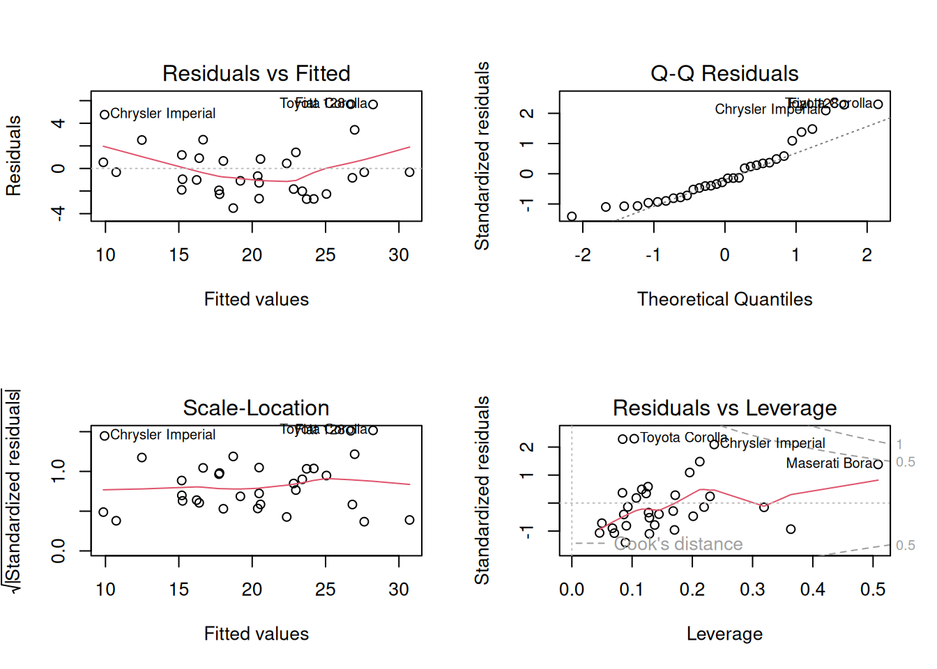
Diagnostics (linearity, normality, leverage)
Influential points (Cook’s distance)
Cook’s distance measures how much the fitted model would change if an observation were removed, combining residual size and leverage.
cd <- cooks.distance(fit_multi)

plot(cd, type = "h", main = "Cook's distance (mtcars)", ylab = "Cook's D")
abline(h = 0, col = "grey60")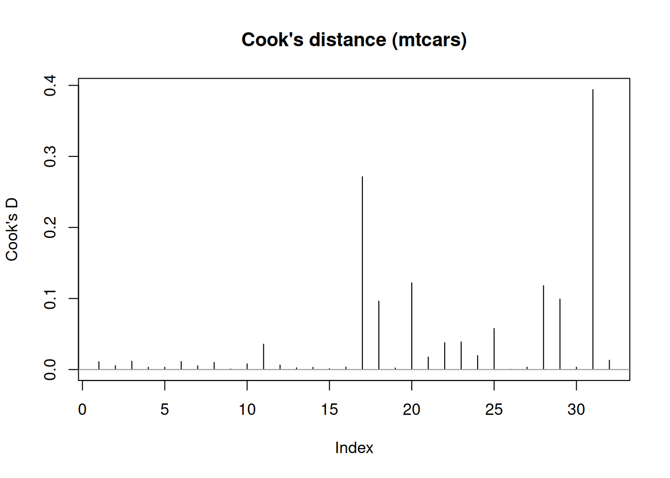
##     Maserati Bora Chrysler Imperial    Toyota Corolla      Lotus Europa
##        0.39406393        0.27133817        0.12213690        0.11810898
##    Ford Pantera L
##        0.09929551
Multicollinearity (VIF)
##     disp       hp     drat       wt
## 8.209402 2.894373 2.279547 5.096601
Rule of thumb: VIF much larger than 5–10 suggests strong collinearity (unstable coefficients).
Heteroscedasticity + robust SE (optional)
# install.packages(c("lmtest", "sandwich"))  # if needed
library(lmtest)
library(sandwich)

bptest(fit_multi)  # Breusch–Pagan test
##
## studentized Breusch-Pagan test
##
## data: fit_multi
## BP = 1.4406, df = 4, p-value = 0.8371##
## t test of coefficients:
##
## Estimate Std. Error t value Pr(>|t|)
## (Intercept) 29.1487376 6.0432074 4.8234 4.896e-05 ***
## disp 0.0038152 0.0082440 0.4628 0.647223
## hp -0.0347835 0.0101670 -3.4212 0.001999 **
## drat 1.7680488 1.0458349 1.6906 0.102435
## wt -3.4796675 1.0993810 -3.1651 0.003819 **
## ---
## Signif. codes: 0 '***' 0.001 '**' 0.01 '*' 0.05 '.' 0.1 ' ' 13) Regression with factors (dummy coding)
With factors, lm() uses a reference level and estimates
coefficients as differences relative to that baseline.
cars_all <- mtcars |>
  mutate(across(c(cyl, vs, am, gear, carb), as.factor))

fit_factors <- lm(mpg ~ ., data = cars_all)
summary(fit_factors)
##
## Call:
## lm(formula = mpg ~ ., data = cars_all)
##
## Residuals:
## Min 1Q Median 3Q Max
## -3.5087 -1.3584 -0.0948 0.7745 4.6251
##
## Coefficients:
## Estimate Std. Error t value Pr(>|t|)
## (Intercept) 23.87913 20.06582 1.190 0.2525
## cyl6 -2.64870 3.04089 -0.871 0.3975
## cyl8 -0.33616 7.15954 -0.047 0.9632
## disp 0.03555 0.03190 1.114 0.2827
## hp -0.07051 0.03943 -1.788 0.0939 .
## drat 1.18283 2.48348 0.476 0.6407
## wt -4.52978 2.53875 -1.784 0.0946 .
## qsec 0.36784 0.93540 0.393 0.6997
## vs1 1.93085 2.87126 0.672 0.5115
## am1 1.21212 3.21355 0.377 0.7113
## gear4 1.11435 3.79952 0.293 0.7733
## gear5 2.52840 3.73636 0.677 0.5089
## carb2 -0.97935 2.31797 -0.423 0.6787
## carb3 2.99964 4.29355 0.699 0.4955
## carb4 1.09142 4.44962 0.245 0.8096
## carb6 4.47757 6.38406 0.701 0.4938
## carb8 7.25041 8.36057 0.867 0.3995
## ---
## Signif. codes: 0 '***' 0.001 '**' 0.01 '*' 0.05 '.' 0.1 ' ' 1
##
## Residual standard error: 2.833 on 15 degrees of freedom
## Multiple R-squared: 0.8931, Adjusted R-squared: 0.779
## F-statistic: 7.83 on 16 and 15 DF, p-value: 0.000124## [1] 32 17## (Intercept) cyl6 cyl8 disp hp drat wt qsec
## Mazda RX4 1 1 0 160 110 3.90 2.620 16.46
## Mazda RX4 Wag 1 1 0 160 110 3.90 2.875 17.02
## Datsun 710 1 0 0 108 93 3.85 2.320 18.61
## Hornet 4 Drive 1 1 0 258 110 3.08 3.215 19.44
## Hornet Sportabout 1 0 1 360 175 3.15 3.440 17.02
## Valiant 1 1 0 225 105 2.76 3.460 20.22Tip: you can change the baseline level via relevel() to
match the interpretation you want.
4) Stepwise regression (AIC) + validation
AIC is defined as \(\mathrm{AIC} = 2k - 2\ln(\hat{L})\), i.e., a trade-off between fit and complexity. Stepwise procedures can be useful for exploration, but they can be unstable and optimistic; good practice is to evaluate performance out-of-sample or via cross-validation.
Stepwise (AIC) in base R
fit_full <- lm(mpg ~ ., data = cars_cont)
fit_null <- lm(mpg ~ 1, data = cars_cont)

fit_step_aic <- step(
  fit_null,
  scope = list(lower = formula(fit_null), upper = formula(fit_full)),
  direction = "both",
  trace = 0
)

summary(fit_step_aic)
##
## Call:
## lm(formula = mpg ~ wt + hp, data = cars_cont)
##
## Residuals:
## Min 1Q Median 3Q Max
## -3.941 -1.600 -0.182 1.050 5.854
##
## Coefficients:
## Estimate Std. Error t value Pr(>|t|)
## (Intercept) 37.22727 1.59879 23.285 < 2e-16 ***
## wt -3.87783 0.63273 -6.129 1.12e-06 ***
## hp -0.03177 0.00903 -3.519 0.00145 **
## ---
## Signif. codes: 0 '***' 0.001 '**' 0.01 '*' 0.05 '.' 0.1 ' ' 1
##
## Residual standard error: 2.593 on 29 degrees of freedom
## Multiple R-squared: 0.8268, Adjusted R-squared: 0.8148
## F-statistic: 69.21 on 2 and 29 DF, p-value: 9.109e-12| df | AIC | |
|---|---|---|
| fit_full | 6 | 158.5837 |
| fit_step_aic | 4 | 156.6523 |
| fit_null | 2 | 208.7555 |
Out-of-sample check (simple train/test RMSE)
set.seed(123)
n <- nrow(cars_cont)
idx_train <- sample.int(n, size = floor(0.8 * n))

train_df <- cars_cont[idx_train, ]
test_df  <- cars_cont[-idx_train, ]

m_full <- lm(mpg ~ ., data = train_df)
m_step <- step(lm(mpg ~ 1, data = train_df),
               scope = list(lower = mpg ~ 1, upper = mpg ~ .),
               direction = "both",
               trace = 0)

rmse <- function(y, yhat) sqrt(mean((y - yhat)^2))

pred_full <- predict(m_full, newdata = test_df)
pred_step <- predict(m_step, newdata = test_df)

c(
  RMSE_full = rmse(test_df$mpg, pred_full),
  RMSE_step = rmse(test_df$mpg, pred_step)
)
## RMSE_full RMSE_step
## 2.049923 4.6047375) Summary table
| Topic | Main_function | Key_outputs | Notes |
|---|---|---|---|
| Simple regression | lm() | Slope/intercept, CI/PI, residuals | Use PI for individual predictions |
| Multiple regression | lm() | t-tests, R^2, diagnostics, VIF, Cook’s D | Check assumptions; consider robust SE if needed |
| Factors | lm() | Reference level, dummy coding, interpretation | Relevel factors to control baseline |
| Model selection | step() + validation | AIC trade-off + out-of-sample RMSE/CV | Stepwise is exploratory; always validate |
A work by Gianluca Sottile
gianluca.sottile@unipa.it