What is a function in R?

A function is a reusable piece of code. It helps you:

avoid repetition,
reduce complexity,
make code easier to test and maintain.

A function can:

take inputs (arguments),
execute a body,
return a value (explicitly with return() or implicitly as the last expression).

Basic syntax:

my_fun <- function(arg1, arg2 = default_value, ...) {
  # body
}

Built-in functions (examples)

R ships with many built-in functions. Arguments can be provided by position or by name, and many arguments have defaults.

diff(): compute differences

diff() is often used in time series workflows to compute lag-1 differences.

set.seed(123)

x <- rnorm(1000)
ts_data <- cumsum(x)

diff_ts <- diff(ts_data)

par(mfrow = c(1, 2))
plot(ts_data, type = "l", main = "Cumulative sum")
plot(diff_ts, type = "l", main = "First differences")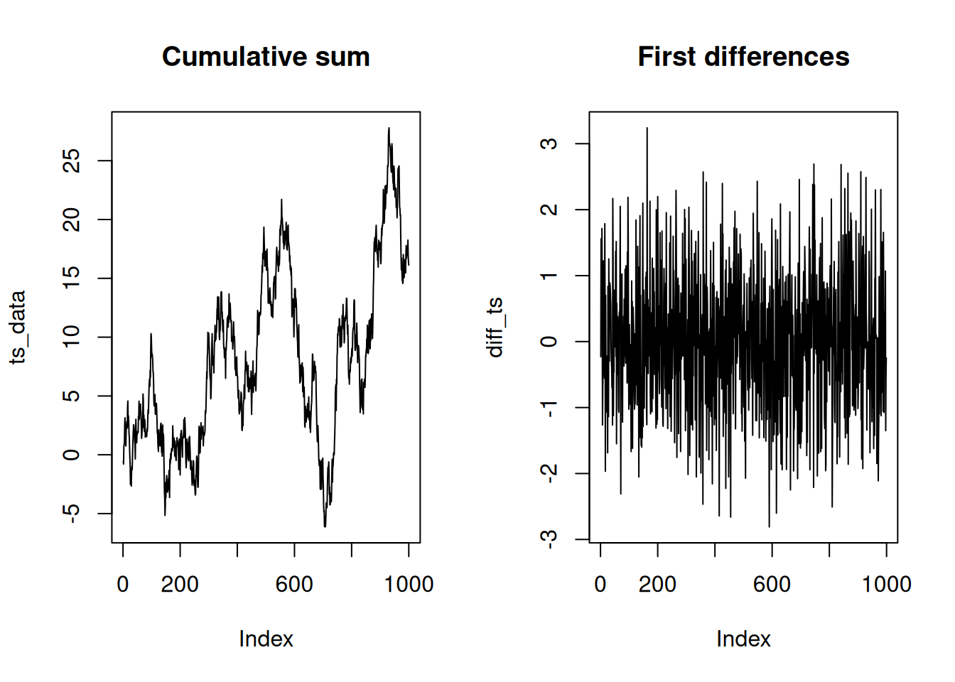

length(): number of elements

length() returns:

number of elements for vectors,
number of columns for data frames/matrices.

data("cars", package = "datasets")

dt <- cars
length(dt)        # number of columns

## [1] 2

nrow(dt)          # number of rows (preferred for data frames)

## [1] 50

length(dt$speed)  # length of a vector

## [1] 50

Math functions

Function	Description
abs(x)	Absolute value
log(x, base = b)	Logarithm (natural log if base is omitted)
exp(x)	Exponential
sqrt(x)	Square root
factorial(x)	Factorial

x_vector <- 1:5
abs(c(-2, 0, 3))

## [1] 2 0 3

log(x_vector)

## [1] 0.0000000 0.6931472 1.0986123 1.3862944 1.6094379

exp(x_vector)

## [1]   2.718282   7.389056  20.085537  54.598150 148.413159

sqrt(x_vector)

## [1] 1.000000 1.414214 1.732051 2.000000 2.236068

factorial(x_vector)

## [1]   1   2   6  24 120

Statistical functions

Function	Description
mean(x)	Mean
median(x)	Median
var(x)	Variance
sd(x)	Standard deviation
scale(x)	Z-scores (standardization)
quantile(x)	Quantiles
summary(x)	Min/1st Qu./Median/Mean/3rd Qu./Max

speed <- dt$speed

mean(speed)

## [1] 15.4

median(speed)

## [1] 15

var(speed)

## [1] 27.95918

sd(speed)

## [1] 5.287644

head(scale(speed), 5)

##           [,1]
## [1,] -2.155969
## [2,] -2.155969
## [3,] -1.588609
## [4,] -1.588609
## [5,] -1.399489

quantile(speed)

##   0%  25%  50%  75% 100% 
##    4   12   15   19   25

summary(speed)

##    Min. 1st Qu.  Median    Mean 3rd Qu.    Max. 
##     4.0    12.0    15.0    15.4    19.0    25.0

Writing your own functions

A user-defined function has:

a name,
arguments (with optional defaults),
a body.

One-argument function

square <- function(n) {
  n^2
}

square(4)

## [1] 16

square(1:5)

## [1]  1  4  9 16 25

If you remove a function, check with exists():

rm(square)
exists("square")

## [1] FALSE

Argument matching (quick demo)

times <- function(x, y) x * y

times(2, 4)          # positional

## [1] 8

times(y = 4, x = 2)  # named (order does not matter)

## [1] 8

Environments and scoping (lexical scoping)

Functions look for variables in their own local environment first; if not found, they search in the environment where the function was created.

y <- 10
f <- function(x) x + y

f(5)   # uses y from outside the function

## [1] 15

## [1] 10

Local variables shadow global ones:

y <- 10
g <- function(x) {
  y <- 100
  x + y
}

g(5)

## [1] 105

## [1] 10

When should you write a function?

If you copy/paste the same logic more than once or twice, it is usually worth writing a function.

Example: normalize to [0, 1]

\[ \text{normalize}(x) = \frac{x - x_{\min}}{x_{\max} - x_{\min}} \]

A robust implementation should handle missing values and constant vectors.

normalize01 <- function(x, na.rm = TRUE) {
  rng <- range(x, na.rm = na.rm)
  denom <- rng[2] - rng[1]

  if (is.na(denom) || denom == 0) {
    return(rep(0, length(x)))
  }

  (x - rng) / denom
}

Apply it to multiple columns with modern syntax:

library(tibble)
library(dplyr)

df_example <- tibble(
  c1 = rnorm(50, 5, 1.5),
  c2 = rnorm(50, 5, 1.5),
  c3 = rnorm(50, 5, 1.5)
)

df_example <- df_example |>
  mutate(across(starts_with("c"), normalize01, .names = "{.col}_norm"))

df_example |> select(ends_with("_norm")) |> head(5)

c1_norm	c2_norm	c3_norm
0.2886787	0.6325447	0.5629538
-0.7195264	-0.4891803	-0.4592776
0.4703763	0.6650164	0.2059713
-0.5508433	-0.6670767	-0.8834820
0.0000000	0.8255361	0.4173301

Functions with conditions: train/test split

A more practical split function usually:

takes a proportion,
optionally takes a seed for reproducibility,
returns both train and test sets.

split_data <- function(df, prop = 0.8, seed = NULL) {
  stopifnot(is.data.frame(df))
  stopifnot(prop > 0 && prop < 1)

  if (!is.null(seed)) set.seed(seed)

  n <- nrow(df)
  n_train <- floor(prop * n)
  idx_train <- sample.int(n, size = n_train)

  list(
    train = df[idx_train, , drop = FALSE],
    test  = df[-idx_train, , drop = FALSE]
  )
}

Test it:

data("airquality", package = "datasets")

spl <- split_data(airquality, prop = 0.8, seed = 123)
dim(spl$train)

## [1] 122   6

dim(spl$test)

## [1] 31  6

A work by Gianluca Sottile

gianluca.sottile@unipa.it

Functions in R Programming