What is ANOVA?

Analysis of Variance (ANOVA) is a statistical method used to test whether the means of two or more groups are equal. ANOVA is an extension of the two-sample t-test to settings with more than two groups.

ANOVA focuses on how the total variability in a numeric outcome can be decomposed into: - Between-group variability (differences between group means), - Within-group variability (variability of observations inside the same group).

One-way ANOVA

A one-way ANOVA compares the means of a numeric variable across levels of a single categorical variable.

Example: a marketing department wants to know whether three teams have the same average sales performance.

Hypotheses

\(H_0\): All group means are equal.
\(H_1\): At least one group mean differs.

Assumptions (typical)

Independent observations.
Approximately normal residuals within each group.
Equal variances across groups (homoscedasticity).

Example: one-way ANOVA with the poisons dataset

We use the poisons dataset:

time: survival time
poison: poison type (3 levels)
treat: treatment type (3 levels)

Step 1) Import and prepare the data

library(dplyr)
library(readr)

path <- "raw_data/poisons.csv"

df <- read_csv(path, show_col_types = FALSE) |>
  # robust: drop index column only if present
  select(-any_of(c("X", "x"))) |>
  mutate(
    poison = factor(poison),
    treat  = factor(treat)
  )

glimpse(df)

## Rows: 48
## Columns: 4
## $ ...1   <dbl> 1, 2, 3, 4, 5, 6, 7, 8, 9, 10, 11, 12, 13, 14, 15, 16, 17, 18, …
## $ time   <dbl> 0.31, 0.45, 0.46, 0.43, 0.36, 0.29, 0.40, 0.23, 0.22, 0.21, 0.1…
## $ poison <fct> 1, 1, 1, 1, 2, 2, 2, 2, 3, 3, 3, 3, 1, 1, 1, 1, 2, 2, 2, 2, 3, …
## $ treat  <fct> A, A, A, A, A, A, A, A, A, A, A, A, B, B, B, B, B, B, B, B, B, …

Step 2) Summary statistics by group

df |>
  dplyr::group_by(poison) |>
  dplyr::summarize(
    n = n(),
    mean_time = mean(time, na.rm = TRUE),
    sd_time = sd(time, na.rm = TRUE),
    .groups = "drop"
  )

poison	n	mean_time	sd_time
1	16	0.617500	0.2094278
2	16	0.544375	0.2893664
3	16	0.276250	0.0622763

Step 3) Visual check (boxplot + jitter)

library(ggplot2)

ggplot(df, aes(x = poison, y = time, fill = poison)) +
  geom_boxplot(alpha = 0.7, width = 0.65, outlier.shape = NA) +
  geom_jitter(width = 0.15, alpha = 0.6, size = 1.6, color = "steelblue") +
  theme_classic() +
  guides(fill = "none")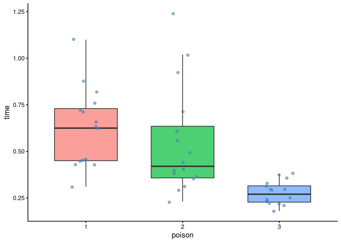

Step 4) Fit the one-way ANOVA

anova_one_way <- aov(time ~ poison, data = df)
summary(anova_one_way)

##             Df Sum Sq Mean Sq F value   Pr(>F)    
## poison       2  1.033  0.5165   11.79 7.66e-05 ***
## Residuals   45  1.972  0.0438                     
## ---
## Signif. codes:  0 '***' 0.001 '**' 0.01 '*' 0.05 '.' 0.1 ' ' 1

Step 5) Post-hoc comparisons (Tukey HSD)

The ANOVA tells you whether any difference exists, but not which pairs differ. Tukey’s HSD provides pairwise comparisons with multiple-testing adjustment.

tukey_one_way <- TukeyHSD(anova_one_way)
tukey_one_way

##   Tukey multiple comparisons of means
##     95% family-wise confidence level
## 
## Fit: aov(formula = time ~ poison, data = df)
## 
## $poison
##          diff        lwr         upr     p adj
## 2-1 -0.073125 -0.2525046  0.10625464 0.5881654
## 3-1 -0.341250 -0.5206296 -0.16187036 0.0000971
## 3-2 -0.268125 -0.4475046 -0.08874536 0.0020924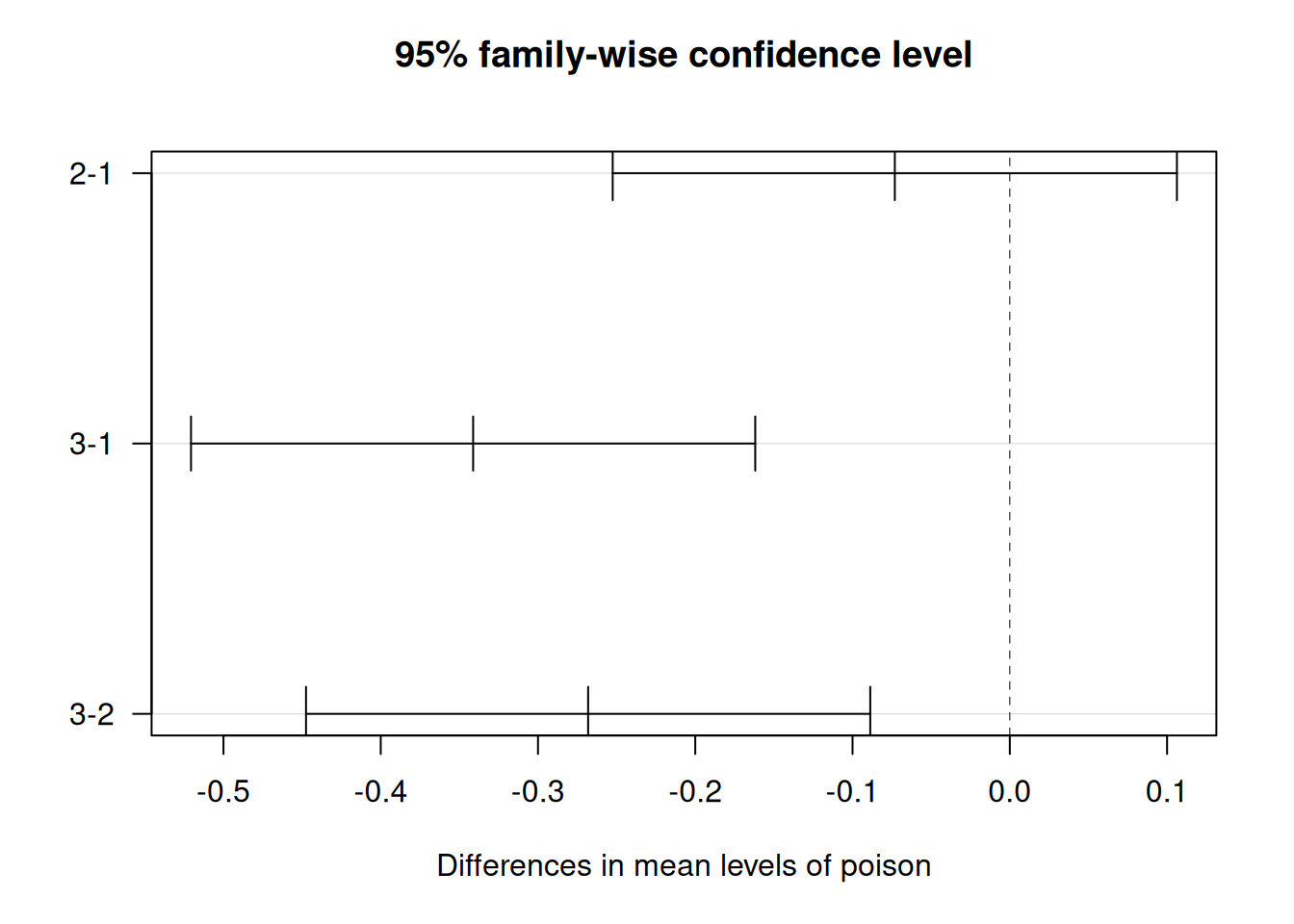

plot(tukey_one_way, las = 1)

Two-way ANOVA

A two-way ANOVA includes two categorical predictors. You typically consider: - Main effects: poison and treat - Interaction: whether the effect of treatment depends on poison type

Additive model (main effects only)

anova_two_way_add <- aov(time ~ poison + treat, data = df)
summary(anova_two_way_add)

##             Df Sum Sq Mean Sq F value  Pr(>F)    
## poison       2 1.0330  0.5165   20.64 5.7e-07 ***
## treat        3 0.9212  0.3071   12.27 6.7e-06 ***
## Residuals   42 1.0509  0.0250                    
## ---
## Signif. codes:  0 '***' 0.001 '**' 0.01 '*' 0.05 '.' 0.1 ' ' 1

Interaction model (recommended to check)

anova_two_way_int <- aov(time ~ poison * treat, data = df)
summary(anova_two_way_int)

##              Df Sum Sq Mean Sq F value   Pr(>F)    
## poison        2 1.0330  0.5165  23.222 3.33e-07 ***
## treat         3 0.9212  0.3071  13.806 3.78e-06 ***
## poison:treat  6 0.2501  0.0417   1.874    0.112    
## Residuals    36 0.8007  0.0222                     
## ---
## Signif. codes:  0 '***' 0.001 '**' 0.01 '*' 0.05 '.' 0.1 ' ' 1

If the interaction term is significant, interpret the interaction first (effects are not constant across levels of the other factor).

Summary

Test	Code
One-way ANOVA	aov(time ~ poison, data = df)
Post-hoc (pairwise)	TukeyHSD(anova_one_way)
Two-way ANOVA (additive)	aov(time ~ poison + treat, data = df)
Two-way ANOVA (interaction)	aov(time ~ poison * treat, data = df)

A work by Gianluca Sottile

gianluca.sottile@unipa.it

ANOVA: One-way & Two-way (with Examples)