DBSCAN (Density-Based Clustering)

DBSCAN groups points based on density rather than distance to centroids. Key concepts:

\(\varepsilon\)-neighborhood: \(N_\varepsilon(x) = \{y: \|x-y\| \le \varepsilon\}\).
Core point: \(|N_\varepsilon(x)| \ge \text{minPts}\).
Border point: not core but density-reachable from a core point.
Noise: points not density-reachable from any core point.

DBSCAN can detect non-spherical clusters and identifies outliers/noise explicitly.

In this lesson

We preprocess business data as in previous lesson.
We choose eps using kNN distance plot.
We run DBSCAN and interpret clusters vs noise.
We compare DBSCAN with K-means on the non-noise subset.

Step 1: Import + preprocessing

library(readr)
library(dplyr)

local_path <- "raw_data/wholesale_customers.csv"

if (!file.exists(local_path)) {
  dir.create("raw_data", showWarnings = FALSE)
  download.file(url_path, local_path, mode = "wb")
}

df_raw <- read_csv(local_path, show_col_types = FALSE)

spend_vars <- c("Fresh", "Milk", "Grocery", "Frozen", "Detergents_Paper", "Delicassen")

X <- df_raw |>
  mutate(across(all_of(spend_vars), ~ log1p(.x))) |>
  select(all_of(spend_vars)) |>
  mutate(across(everything(), scale)) |>
  as.data.frame()

Step 2: Parameter selection (minPts and eps)

A common heuristic sets \(\text{minPts} \approx 2p\) where \(p\) is the number of features.

p <- ncol(X)
minPts <- max(5, 2 * p)
minPts

## [1] 12

To choose eps, inspect the kNN distance plot: pick eps near the “knee”.

library(dbscan)

kNNdistplot(X, k = minPts)
abline(h = 1, col = "red", lty = 2)

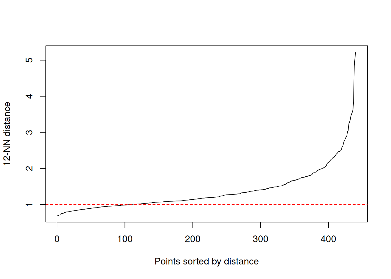
Replace the horizontal line with your candidate value for eps after inspecting the knee.

Step 3: Fit DBSCAN

eps <- 1.0  # adjust after inspecting the kNN plot

db <- dbscan(X, eps = eps, minPts = minPts)
db

## DBSCAN clustering for 440 objects.
## Parameters: eps = 1, minPts = 12
## Using euclidean distances and borderpoints = TRUE
## The clustering contains 1 cluster(s) and 182 noise points.
## 
##   0   1 
## 182 258 
## 
## Available fields: cluster, eps, minPts, metric, borderPoints

table(db$cluster)  # 0 = noise

## 
##   0   1 
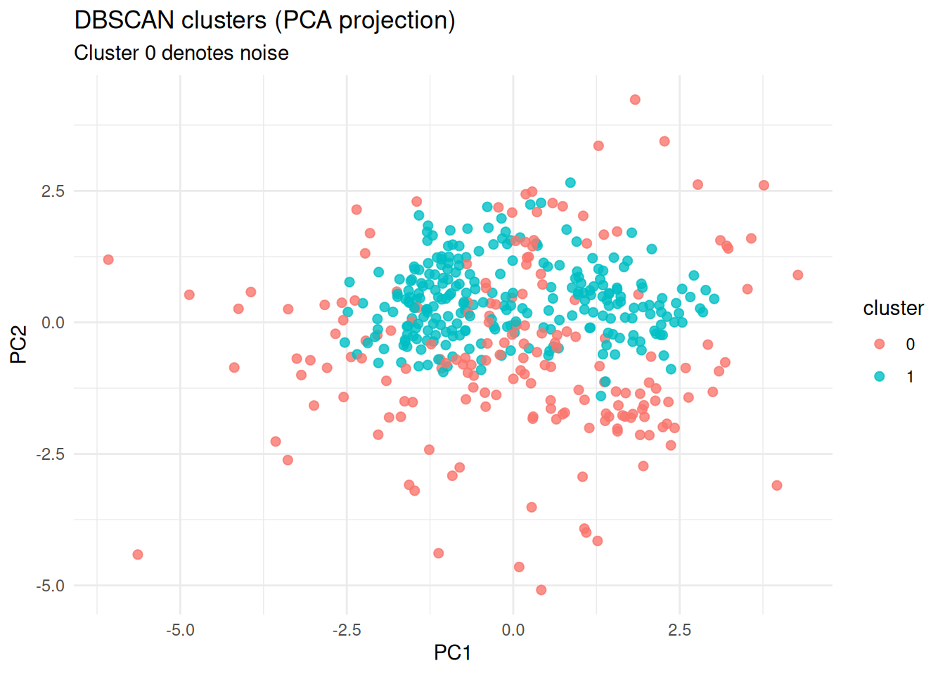
## 182 258

Interpretation: - If most points are noise, eps may be too small or minPts too large. - If almost no noise and very few clusters, eps may be too large (merging structures).

Step 4: Visualization (PCA projection)

library(ggplot2)

pc <- prcomp(X)
plot_df <- data.frame(
  PC1 = pc$x[, 1],
  PC2 = pc$x[, 2],
  cluster = factor(db$cluster)
)

ggplot(plot_df, aes(PC1, PC2, color = cluster)) +
  geom_point(alpha = 0.8, size = 2) +
  theme_minimal() +
  labs(
    title = "DBSCAN clusters (PCA projection)",
    subtitle = "Cluster 0 denotes noise",
    x = "PC1", y = "PC2"
  )

Step 5: Internal validation (silhouette on non-noise points)

Silhouette is not directly defined for noise. A practical approach is to compute silhouette on the subset with cluster label \(\ge 1\).

library(cluster)

idx <- which(db$cluster > 0)
X_nonoise <- X[idx, , drop = FALSE]
cl_nonoise <- db$cluster[idx]

if (length(unique(cl_nonoise)) >= 2) {
  d <- dist(X_nonoise)
  sil <- silhouette(cl_nonoise, d)
  summary(sil)
  plot(sil, border = NA, main = "Silhouette (non-noise subset)")
}

Step 6: Comparison with K-means (on non-noise subset)

library(mclust)

k_db <- length(unique(cl_nonoise))
set.seed(123)
km <- kmeans(X_nonoise, centers = k_db, nstart = 50)

ari <- adjustedRandIndex(cl_nonoise, km$cluster)
ari

## [1] 1

Interpretation:

Agreement is not expected to be perfect, because DBSCAN optimizes density connectivity, not SSE.
Differences often highlight non-spherical structure or outliers.

Step 7: Practical reporting

For a business segmentation report:

Report number of clusters found (excluding noise) and proportion of noise.
Provide cluster profiles (feature means in original units, not only z-scores).
Explain that DBSCAN can isolate atypical customers as noise/outliers, which may be a feature rather than a drawback.

Summary

DBSCAN is density-based and can recover non-spherical clusters.
minPts and eps are critical; the kNN distance plot is a practical tool for selecting eps.
Noise labeling provides a principled way to treat outliers.
Compare with K-means on the non-noise subset to understand structural differences.

A work by Gianluca Sottile

gianluca.sottile@unipa.it

DBSCAN in R — eps, minPts, Noise Handling, and Non-spherical Clusters