Gradient Boosting Machines (GBM) — XGBoost

Gradient Boosting builds an ensemble \(F_M(x) = \sum_{m=1}^M T_m(x)\) by functional gradient descent: each tree \(T_m\) fits pseudo-residuals \(r_{im} = -[\mathcal{L}(y_i, F_{m-1}(x_i))]\) of the base learner loss \(\mathcal{L}\) (logistic \(logloss\) here), with regularization:

\[ \mathcal{L} = - \sum [y_i \log p_i + (1-y_i)\log(1-p_i)] + \Omega(F) \]

XGBoost adds L1/L2 tree regularization, subsampling, early stopping. Extremely efficient (histogram binning, sparsity-aware).

Lesson: Complete pipeline on Titanic (\(n=1309\), 38% survival), CV tuning, SHAP importance.

Step 1: Data import & EDA

library(dplyr)
path <- "raw_data/titanic_data.csv"
titanic <- read.csv(path, stringsAsFactors = FALSE)

dim(titanic)

## [1] 1309   13

prop.table(table(titanic$survived))  # 38% Yes (imbalanced)

## 
##        0        1 
## 0.618029 0.381971

head(titanic)

x	pclass	survived	name	sex	age	sibsp	parch	ticket	fare	cabin	embarked	home.dest
1	1	1	Allen, Miss. Elisabeth Walton	female	29	0	0	24160	211.3375	B5	S	St Louis, MO
2	1	1	Allison, Master. Hudson Trevor	male	0.9167	1	2	113781	151.55	C22 C26	S	Montreal, PQ / Chesterville, ON
3	1	0	Allison, Miss. Helen Loraine	female	2	1	2	113781	151.55	C22 C26	S	Montreal, PQ / Chesterville, ON
4	1	0	Allison, Mr. Hudson Joshua Creighton	male	30	1	2	113781	151.55	C22 C26	S	Montreal, PQ / Chesterville, ON
5	1	0	Allison, Mrs. Hudson J C (Bessie Waldo Daniels)	female	25	1	2	113781	151.55	C22 C26	S	Montreal, PQ / Chesterville, ON
6	1	1	Anderson, Mr. Harry	male	48	0	0	19952	26.55	E12	S	New York, NY

Step 2: Feature engineering & encoding

titanic_clean <- titanic |>
  select(-any_of(c("home.dest", "cabin", "name", "X", "x", "ticket"))) |>
  filter(embarked != "?") |>
  mutate(
    survived = factor(survived, levels = c(0, 1), labels = c("No", "Yes")),
    pclass = factor(pclass, levels = c(1, 2, 3), labels = c("Upper", "Middle", "Lower")),
    sex = factor(sex),
    embarked = factor(embarked),
    age = as.numeric(age),
    fare = as.numeric(fare),
    sibsp = as.numeric(sibsp),
    parch = as.numeric(parch),
    family_size = sibsp + parch + 1,
    age_child = ifelse(age < 18, 1, 0),  # interaction
    fare_log = log(fare + 1)
  ) |>
  na.omit()

glimpse(titanic_clean)

## Rows: 1,043
## Columns: 11
## $ pclass      <fct> Upper, Upper, Upper, Upper, Upper, Upper, Upper, Upper, Up…
## $ survived    <fct> Yes, Yes, No, No, No, Yes, Yes, No, Yes, No, No, Yes, Yes,…
## $ sex         <fct> female, male, female, male, female, male, female, male, fe…
## $ age         <dbl> 29.0000, 0.9167, 2.0000, 30.0000, 25.0000, 48.0000, 63.000…
## $ sibsp       <dbl> 0, 1, 1, 1, 1, 0, 1, 0, 2, 0, 1, 1, 0, 0, 0, 0, 0, 0, 0, 1…
## $ parch       <dbl> 0, 2, 2, 2, 2, 0, 0, 0, 0, 0, 0, 0, 0, 0, 0, 1, 1, 0, 0, 1…
## $ fare        <dbl> 211.3375, 151.5500, 151.5500, 151.5500, 151.5500, 26.5500,…
## $ embarked    <fct> S, S, S, S, S, S, S, S, S, C, C, C, C, S, S, C, C, C, C, S…
## $ family_size <dbl> 1, 4, 4, 4, 4, 1, 2, 1, 3, 1, 2, 2, 1, 1, 1, 2, 2, 1, 1, 3…
## $ age_child   <dbl> 0, 1, 1, 0, 0, 0, 0, 0, 0, 0, 0, 0, 0, 0, 0, 0, 0, 0, 0, 0…
## $ fare_log    <dbl> 5.358177, 5.027492, 5.027492, 5.027492, 5.027492, 3.316003…

XGBoost DMatrix (numeric + labels 0/1):

X_all <- model.matrix(survived ~ . - 1, data = titanic_clean)
y_all <- as.numeric(titanic_clean$survived == "Yes")  # 0/1 numeric

dim(X_all)

## [1] 1043   13

Step 3: Train/valid/test split (70/15/15)

library(xgboost)

set.seed(123)
n <- nrow(X_all)
idx_train <- sample(n, floor(0.7 * n))
idx_rem <- setdiff(1:n, idx_train)
idx_valid <- sample(idx_rem, floor(0.15 * n))

X_train <- X_all[idx_train, ]; y_train <- y_all[idx_train]
X_valid <- X_all[idx_valid, ]; y_valid <- y_all[idx_valid]
X_test  <- X_all[-c(idx_train, idx_valid), ]; y_test  <- y_all[-c(idx_train, idx_valid)]

dtrain <- xgb.DMatrix(X_train, label = y_train)
dvalid <- xgb.DMatrix(X_valid, label = y_valid)
dtest  <- xgb.DMatrix(X_test,  label = y_test)

Step 4: Baseline model (logloss objective)

library(pROC)

params_base <- list(
  objective = "binary:logistic",
  eval_metric = c("logloss", "auc", "error"),
  booster = "gbtree",
  max_depth = 4,
  eta = 0.1,                    # learning rate
  subsample = 0.8,              # row sampling
  colsample_bytree = 0.8,       # column sampling
  lambda = 1,                   # L2 regularization
  alpha = 0                     # L1 regularization
)

set.seed(123)
xgb_base <- xgb.train(
  params = params_base,
  data = dtrain,
  nrounds = 500,
  watchlist = list(train = dtrain, valid = dvalid),
  early_stopping_rounds = 30,
  verbose = 1,
  maximize = FALSE
)

## Multiple eval metrics are present. Will use valid_error for early stopping.
## Will train until valid_error hasn't improved in 30 rounds.
## 
## [1]  train-logloss:0.659355  train-auc:0.761805  train-error:0.417808    valid-logloss:0.651729  valid-auc:0.748713  valid-error:0.397436 
## [2]  train-logloss:0.622657  train-auc:0.867013  train-error:0.332877    valid-logloss:0.613583  valid-auc:0.897049  valid-error:0.326923 
## [3]  train-logloss:0.591894  train-auc:0.873828  train-error:0.243836    valid-logloss:0.581692  valid-auc:0.903912  valid-error:0.237179 
## [4]  train-logloss:0.581913  train-auc:0.876818  train-error:0.236986    valid-logloss:0.573698  valid-auc:0.898164  valid-error:0.230769 
## [5]  train-logloss:0.558866  train-auc:0.881072  train-error:0.186301    valid-logloss:0.549989  valid-auc:0.895333  valid-error:0.185897 
## [6]  train-logloss:0.549253  train-auc:0.884008  train-error:0.182192    valid-logloss:0.545676  valid-auc:0.884351  valid-error:0.198718 
## [7]  train-logloss:0.529660  train-auc:0.887090  train-error:0.176712    valid-logloss:0.524362  valid-auc:0.890100  valid-error:0.179487 
## [8]  train-logloss:0.512308  train-auc:0.891850  train-error:0.175342    valid-logloss:0.509222  valid-auc:0.889327  valid-error:0.179487 
## [9]  train-logloss:0.498081  train-auc:0.892856  train-error:0.175342    valid-logloss:0.494742  valid-auc:0.888126  valid-error:0.179487 
## [10] train-logloss:0.492402  train-auc:0.894542  train-error:0.178082    valid-logloss:0.490760  valid-auc:0.889842  valid-error:0.173077 
## [11] train-logloss:0.480442  train-auc:0.896486  train-error:0.173973    valid-logloss:0.476706  valid-auc:0.893102  valid-error:0.179487 
## [12] train-logloss:0.468971  train-auc:0.896984  train-error:0.175342    valid-logloss:0.463746  valid-auc:0.897049  valid-error:0.179487 
## [13] train-logloss:0.458830  train-auc:0.897732  train-error:0.173973    valid-logloss:0.454623  valid-auc:0.893960  valid-error:0.179487 
## [14] train-logloss:0.454564  train-auc:0.899448  train-error:0.176712    valid-logloss:0.452513  valid-auc:0.892330  valid-error:0.179487 
## [15] train-logloss:0.447081  train-auc:0.898442  train-error:0.169863    valid-logloss:0.445189  valid-auc:0.892416  valid-error:0.173077 
## [16] train-logloss:0.439481  train-auc:0.898642  train-error:0.168493    valid-logloss:0.437798  valid-auc:0.894647  valid-error:0.160256 
## [17] train-logloss:0.433263  train-auc:0.900540  train-error:0.168493    valid-logloss:0.432862  valid-auc:0.892244  valid-error:0.160256 
## [18] train-logloss:0.427947  train-auc:0.901508  train-error:0.167123    valid-logloss:0.429246  valid-auc:0.892073  valid-error:0.173077 
## [19] train-logloss:0.423983  train-auc:0.904378  train-error:0.167123    valid-logloss:0.429559  valid-auc:0.891644  valid-error:0.173077 
## [20] train-logloss:0.420375  train-auc:0.905844  train-error:0.167123    valid-logloss:0.427414  valid-auc:0.889928  valid-error:0.166667 
## [21] train-logloss:0.417052  train-auc:0.907244  train-error:0.165753    valid-logloss:0.426086  valid-auc:0.890957  valid-error:0.160256 
## [22] train-logloss:0.412216  train-auc:0.908629  train-error:0.165753    valid-logloss:0.421541  valid-auc:0.891558  valid-error:0.166667 
## [23] train-logloss:0.409860  train-auc:0.909878  train-error:0.168493    valid-logloss:0.419983  valid-auc:0.890872  valid-error:0.166667 
## [24] train-logloss:0.405229  train-auc:0.910492  train-error:0.164384    valid-logloss:0.419276  valid-auc:0.890014  valid-error:0.166667 
## [25] train-logloss:0.401842  train-auc:0.910623  train-error:0.164384    valid-logloss:0.413739  valid-auc:0.892759  valid-error:0.173077 
## [26] train-logloss:0.397486  train-auc:0.913211  train-error:0.164384    valid-logloss:0.413149  valid-auc:0.890357  valid-error:0.179487 
## [27] train-logloss:0.396177  train-auc:0.913747  train-error:0.160274    valid-logloss:0.413045  valid-auc:0.888984  valid-error:0.173077 
## [28] train-logloss:0.393186  train-auc:0.913612  train-error:0.161644    valid-logloss:0.411055  valid-auc:0.889671  valid-error:0.173077 
## [29] train-logloss:0.389146  train-auc:0.914581  train-error:0.160274    valid-logloss:0.410768  valid-auc:0.889327  valid-error:0.179487 
## [30] train-logloss:0.385807  train-auc:0.915198  train-error:0.157534    valid-logloss:0.409788  valid-auc:0.890528  valid-error:0.179487 
## [31] train-logloss:0.382588  train-auc:0.916640  train-error:0.156164    valid-logloss:0.409580  valid-auc:0.890528  valid-error:0.166667 
## [32] train-logloss:0.379137  train-auc:0.918191  train-error:0.157534    valid-logloss:0.409297  valid-auc:0.889327  valid-error:0.166667 
## [33] train-logloss:0.377047  train-auc:0.918677  train-error:0.156164    valid-logloss:0.409548  valid-auc:0.888813  valid-error:0.179487 
## [34] train-logloss:0.375292  train-auc:0.919418  train-error:0.154795    valid-logloss:0.410409  valid-auc:0.888298  valid-error:0.173077 
## [35] train-logloss:0.372804  train-auc:0.921153  train-error:0.154795    valid-logloss:0.409958  valid-auc:0.887612  valid-error:0.173077 
## [36] train-logloss:0.370564  train-auc:0.920914  train-error:0.152055    valid-logloss:0.411016  valid-auc:0.886925  valid-error:0.173077 
## [37] train-logloss:0.368003  train-auc:0.921643  train-error:0.153425    valid-logloss:0.411909  valid-auc:0.887268  valid-error:0.179487 
## [38] train-logloss:0.366152  train-auc:0.921400  train-error:0.153425    valid-logloss:0.411374  valid-auc:0.886754  valid-error:0.179487 
## [39] train-logloss:0.363723  train-auc:0.922943  train-error:0.150685    valid-logloss:0.412208  valid-auc:0.886067  valid-error:0.179487 
## [40] train-logloss:0.360854  train-auc:0.924617  train-error:0.149315    valid-logloss:0.412796  valid-auc:0.887440  valid-error:0.179487 
## [41] train-logloss:0.358494  train-auc:0.926438  train-error:0.149315    valid-logloss:0.414552  valid-auc:0.887268  valid-error:0.179487 
## [42] train-logloss:0.357058  train-auc:0.926457  train-error:0.149315    valid-logloss:0.413268  valid-auc:0.886925  valid-error:0.173077 
## [43] train-logloss:0.354799  train-auc:0.927205  train-error:0.147945    valid-logloss:0.413334  valid-auc:0.885810  valid-error:0.179487 
## [44] train-logloss:0.352786  train-auc:0.927977  train-error:0.147945    valid-logloss:0.413864  valid-auc:0.883922  valid-error:0.179487 
## [45] train-logloss:0.350757  train-auc:0.929057  train-error:0.146575    valid-logloss:0.412470  valid-auc:0.885295  valid-error:0.173077 
## Stopping. Best iteration:
## [46] train-logloss:0.349447  train-auc:0.929254  train-error:0.146575    valid-logloss:0.411607  valid-auc:0.886496  valid-error:0.179487
## 
## [46] train-logloss:0.349447  train-auc:0.929254  train-error:0.146575    valid-logloss:0.411607  valid-auc:0.886496  valid-error:0.179487

xgb_base$best_score  # best logloss

## NULL

Early stopping at round ~40: Prevents overfitting.

Step 5: Predictions & confusion matrix

pred_test_prob <- predict(xgb_base, dtest)
pred_test_class <- as.numeric(pred_test_prob > 0.5)

cm <- table(Actual = y_test, Predicted = pred_test_class)
print(cm)

##       Predicted
## Actual  0  1
##      0 88 11
##      1 17 41

(accuracy <- sum(diag(cm)) / sum(cm))

## [1] 0.8216561

Sensitivity/Specificity (threshold 0.5):

sensitivity <- cm[2,2] / sum(cm[2,])
specificity <- cm[1,1] / sum(cm[1,])
c(Sens = round(sensitivity, 3), Spec = round(specificity, 3))

##  Sens  Spec 
## 0.707 0.889

Step 6: ROC curve

roc_obj <- roc(y_test, pred_test_prob, quiet = TRUE)
plot(roc_obj, main = "XGBoost ROC — Titanic Test", print.auc = TRUE, print.thres = "best")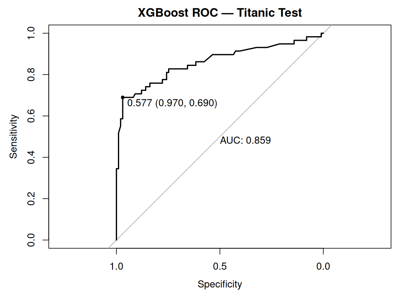

AUC 0.84–0.86: Excellent discrimination despite imbalance.

Step 7: Cross-validation + early stopping (optimal nrounds)

set.seed(123)
cv_xgb <- xgb.cv(
  params = params_base,
  data = dtrain,
  nrounds = 2000,
  nfold = 5,
  stratified = TRUE,           # preserve class balance
  early_stopping_rounds = 50,
  verbose = 1,
  maximize = FALSE
)

## Multiple eval metrics are present. Will use test_error for early stopping.
## Will train until test_error hasn't improved in 50 rounds.
## 
## [1]  train-logloss:0.659842±0.003449 train-auc:0.756650±0.019298 train-error:0.417808±0.002422   test-logloss:0.666899±0.006810  test-auc:0.682059±0.047251  test-error:0.417808±0.009686 
## [2]  train-logloss:0.623586±0.004396 train-auc:0.868269±0.005635 train-error:0.344863±0.022148   test-logloss:0.636146±0.010129  test-auc:0.800559±0.052951  test-error:0.353425±0.030860 
## [3]  train-logloss:0.592606±0.005155 train-auc:0.881629±0.006757 train-error:0.234589±0.017836   test-logloss:0.608977±0.013955  test-auc:0.828870±0.049839  test-error:0.265753±0.039465 
## [4]  train-logloss:0.567908±0.006368 train-auc:0.883746±0.007453 train-error:0.203082±0.015248   test-logloss:0.587132±0.015748  test-auc:0.838711±0.045388  test-error:0.242466±0.035126 
## [5]  train-logloss:0.546742±0.007134 train-auc:0.883880±0.008322 train-error:0.183562±0.014296   test-logloss:0.569055±0.017965  test-auc:0.841737±0.041495  test-error:0.224658±0.033694 
## [6]  train-logloss:0.528091±0.007803 train-auc:0.884730±0.005905 train-error:0.183219±0.013591   test-logloss:0.554054±0.019845  test-auc:0.840224±0.045198  test-error:0.223288±0.035458 
## [7]  train-logloss:0.510856±0.008901 train-auc:0.888454±0.004922 train-error:0.179795±0.015879   test-logloss:0.539281±0.021213  test-auc:0.846828±0.041142  test-error:0.212329±0.036885 
## [8]  train-logloss:0.496335±0.009512 train-auc:0.890749±0.005931 train-error:0.177397±0.016272   test-logloss:0.529117±0.023304  test-auc:0.847193±0.039148  test-error:0.213699±0.036372 
## [9]  train-logloss:0.483910±0.010394 train-auc:0.892845±0.006095 train-error:0.176027±0.014898   test-logloss:0.521041±0.025402  test-auc:0.847164±0.039876  test-error:0.216438±0.036757 
## [10] train-logloss:0.472797±0.010203 train-auc:0.894075±0.006344 train-error:0.174315±0.013341   test-logloss:0.512574±0.027618  test-auc:0.849265±0.040674  test-error:0.209589±0.040405 
## [11] train-logloss:0.462374±0.010837 train-auc:0.895601±0.005957 train-error:0.174658±0.015600   test-logloss:0.504878±0.028834  test-auc:0.850506±0.041564  test-error:0.219178±0.044124 
## [12] train-logloss:0.453564±0.011263 train-auc:0.897925±0.006798 train-error:0.172945±0.013319   test-logloss:0.498713±0.031411  test-auc:0.850047±0.041620  test-error:0.216438±0.046100 
## [13] train-logloss:0.445588±0.011050 train-auc:0.899252±0.005540 train-error:0.170205±0.012618   test-logloss:0.493730±0.032879  test-auc:0.849571±0.042441  test-error:0.217808±0.052477 
## [14] train-logloss:0.437733±0.011391 train-auc:0.900846±0.006022 train-error:0.169178±0.013007   test-logloss:0.489675±0.033713  test-auc:0.850310±0.040842  test-error:0.221918±0.048818 
## [15] train-logloss:0.430860±0.011208 train-auc:0.902953±0.005291 train-error:0.167808±0.009686   test-logloss:0.485968±0.036417  test-auc:0.851696±0.040897  test-error:0.221918±0.051393 
## [16] train-logloss:0.426158±0.011390 train-auc:0.906040±0.005751 train-error:0.166781±0.010101   test-logloss:0.482746±0.036821  test-auc:0.852559±0.040227  test-error:0.219178±0.051484 
## [17] train-logloss:0.420078±0.011513 train-auc:0.907355±0.006083 train-error:0.165068±0.010597   test-logloss:0.479641±0.037780  test-auc:0.853211±0.039399  test-error:0.215068±0.044283 
## [18] train-logloss:0.415387±0.011415 train-auc:0.908271±0.005895 train-error:0.163699±0.008781   test-logloss:0.476781±0.038349  test-auc:0.853622±0.039103  test-error:0.213699±0.049722 
## [19] train-logloss:0.410502±0.011713 train-auc:0.908886±0.006306 train-error:0.163014±0.008681   test-logloss:0.473789±0.039855  test-auc:0.854546±0.039578  test-error:0.216438±0.052744 
## [20] train-logloss:0.406882±0.012554 train-auc:0.911035±0.007273 train-error:0.161986±0.008527   test-logloss:0.473626±0.040559  test-auc:0.852176±0.040774  test-error:0.219178±0.052163 
## [21] train-logloss:0.403567±0.012408 train-auc:0.913143±0.006274 train-error:0.157877±0.008681   test-logloss:0.473638±0.041368  test-auc:0.852280±0.041438  test-error:0.223288±0.051620 
## [22] train-logloss:0.399943±0.012485 train-auc:0.913671±0.005869 train-error:0.158562±0.009881   test-logloss:0.472971±0.043167  test-auc:0.851487±0.040299  test-error:0.223288±0.055980 
## [23] train-logloss:0.395854±0.012342 train-auc:0.915480±0.005640 train-error:0.156507±0.013515   test-logloss:0.470606±0.043381  test-auc:0.853228±0.040963  test-error:0.221918±0.054709 
## [24] train-logloss:0.392065±0.011866 train-auc:0.916602±0.005747 train-error:0.154795±0.011777   test-logloss:0.468587±0.044124  test-auc:0.853460±0.041103  test-error:0.216438±0.052298 
## [25] train-logloss:0.388179±0.011730 train-auc:0.917258±0.005369 train-error:0.153082±0.011651   test-logloss:0.466868±0.043903  test-auc:0.853804±0.040666  test-error:0.217808±0.056977 
## [26] train-logloss:0.384919±0.011175 train-auc:0.918233±0.005818 train-error:0.153082±0.012734   test-logloss:0.466492±0.046533  test-auc:0.853767±0.040724  test-error:0.220548±0.051802 
## [27] train-logloss:0.382493±0.011626 train-auc:0.919145±0.005668 train-error:0.152397±0.012168   test-logloss:0.466581±0.047542  test-auc:0.853889±0.041911  test-error:0.219178±0.052387 
## [28] train-logloss:0.379403±0.011467 train-auc:0.919985±0.005538 train-error:0.151027±0.012431   test-logloss:0.465205±0.048187  test-auc:0.854697±0.041202  test-error:0.220548±0.049248 
## [29] train-logloss:0.376638±0.011429 train-auc:0.921659±0.005866 train-error:0.148630±0.011702   test-logloss:0.464798±0.048883  test-auc:0.854263±0.042042  test-error:0.220548±0.047056 
## [30] train-logloss:0.373989±0.011549 train-auc:0.922487±0.005727 train-error:0.147260±0.014580   test-logloss:0.463914±0.049431  test-auc:0.854690±0.042255  test-error:0.223288±0.047106 
## [31] train-logloss:0.371522±0.011618 train-auc:0.923397±0.005699 train-error:0.146575±0.012383   test-logloss:0.463226±0.049597  test-auc:0.855576±0.041967  test-error:0.217808±0.051802 
## [32] train-logloss:0.369128±0.011502 train-auc:0.924625±0.005137 train-error:0.148630±0.013666   test-logloss:0.463716±0.051130  test-auc:0.855027±0.042778  test-error:0.219178±0.046454 
## [33] train-logloss:0.366634±0.011622 train-auc:0.925006±0.004997 train-error:0.146575±0.012084   test-logloss:0.463228±0.051696  test-auc:0.855024±0.041839  test-error:0.219178±0.053495 
## [34] train-logloss:0.363754±0.011657 train-auc:0.926509±0.005824 train-error:0.148630±0.012606   test-logloss:0.463294±0.050510  test-auc:0.854709±0.040633  test-error:0.217808±0.054666 
## [35] train-logloss:0.361063±0.011441 train-auc:0.927220±0.005419 train-error:0.146918±0.011826   test-logloss:0.462902±0.052072  test-auc:0.854514±0.040461  test-error:0.213699±0.058199 
## [36] train-logloss:0.358713±0.011675 train-auc:0.928062±0.005669 train-error:0.144863±0.011839   test-logloss:0.463192±0.053556  test-auc:0.853212±0.042507  test-error:0.217808±0.057591 
## [37] train-logloss:0.356415±0.011318 train-auc:0.928856±0.005503 train-error:0.142466±0.012011   test-logloss:0.463206±0.054406  test-auc:0.852747±0.042100  test-error:0.219178±0.062588 
## [38] train-logloss:0.354517±0.011207 train-auc:0.929490±0.005350 train-error:0.142466±0.012312   test-logloss:0.462625±0.054574  test-auc:0.852630±0.042716  test-error:0.216438±0.058239 
## [39] train-logloss:0.352631±0.010974 train-auc:0.929936±0.005230 train-error:0.140411±0.010274   test-logloss:0.462686±0.055864  test-auc:0.852347±0.043867  test-error:0.219178±0.058920 
## [40] train-logloss:0.351009±0.011053 train-auc:0.930155±0.005154 train-error:0.140753±0.010789   test-logloss:0.462369±0.056232  test-auc:0.853199±0.043874  test-error:0.220548±0.059985 
## [41] train-logloss:0.349448±0.010778 train-auc:0.930955±0.004633 train-error:0.139384±0.009881   test-logloss:0.462714±0.055837  test-auc:0.852481±0.043155  test-error:0.219178±0.057713 
## [42] train-logloss:0.347900±0.010911 train-auc:0.931843±0.004697 train-error:0.139384±0.009269   test-logloss:0.462338±0.055917  test-auc:0.852478±0.042861  test-error:0.220548±0.059985 
## [43] train-logloss:0.346335±0.011616 train-auc:0.932567±0.005136 train-error:0.139384±0.008613   test-logloss:0.462352±0.055812  test-auc:0.852515±0.042375  test-error:0.217808±0.053801 
## [44] train-logloss:0.344335±0.012000 train-auc:0.933524±0.005242 train-error:0.138356±0.009173   test-logloss:0.462709±0.056260  test-auc:0.853003±0.042845  test-error:0.220548±0.051118 
## [45] train-logloss:0.342801±0.012152 train-auc:0.934218±0.005158 train-error:0.137329±0.009940   test-logloss:0.462550±0.056304  test-auc:0.852737±0.042998  test-error:0.220548±0.053582 
## [46] train-logloss:0.340842±0.011761 train-auc:0.935292±0.005038 train-error:0.138699±0.008731   test-logloss:0.464328±0.055652  test-auc:0.852364±0.041811  test-error:0.226027±0.051256 
## [47] train-logloss:0.339171±0.012100 train-auc:0.936262±0.005330 train-error:0.138356±0.009410   test-logloss:0.464815±0.055570  test-auc:0.851548±0.040749  test-error:0.223288±0.051393 
## [48] train-logloss:0.337883±0.011656 train-auc:0.936310±0.005013 train-error:0.137671±0.009269   test-logloss:0.463714±0.054799  test-auc:0.851931±0.040260  test-error:0.223288±0.051393 
## [49] train-logloss:0.336558±0.011652 train-auc:0.936955±0.005059 train-error:0.137671±0.010388   test-logloss:0.463573±0.054129  test-auc:0.851775±0.039733  test-error:0.224658±0.050192 
## [50] train-logloss:0.335299±0.011458 train-auc:0.937430±0.004805 train-error:0.135616±0.009866   test-logloss:0.463445±0.054454  test-auc:0.851775±0.040294  test-error:0.223288±0.051847 
## [51] train-logloss:0.333683±0.011227 train-auc:0.938249±0.004779 train-error:0.134589±0.010870   test-logloss:0.463592±0.056010  test-auc:0.852455±0.041583  test-error:0.224658±0.046806 
## [52] train-logloss:0.332073±0.011468 train-auc:0.938993±0.005005 train-error:0.132534±0.011525   test-logloss:0.463681±0.055254  test-auc:0.853191±0.040686  test-error:0.224658±0.049958 
## [53] train-logloss:0.329897±0.011512 train-auc:0.939813±0.005039 train-error:0.131164±0.011839   test-logloss:0.463461±0.054948  test-auc:0.852764±0.040295  test-error:0.223288±0.047847 
## [54] train-logloss:0.328446±0.011669 train-auc:0.940203±0.005183 train-error:0.130822±0.012734   test-logloss:0.463389±0.054860  test-auc:0.853380±0.040430  test-error:0.221918±0.048818 
## [55] train-logloss:0.327339±0.011631 train-auc:0.940874±0.004969 train-error:0.130137±0.012814   test-logloss:0.463313±0.055030  test-auc:0.852956±0.040021  test-error:0.221918±0.045844 
## [56] train-logloss:0.325684±0.011841 train-auc:0.941607±0.004741 train-error:0.128767±0.011950   test-logloss:0.463207±0.055445  test-auc:0.853459±0.040171  test-error:0.221918±0.043210 
## [57] train-logloss:0.324078±0.012114 train-auc:0.942318±0.004918 train-error:0.127055±0.011764   test-logloss:0.464121±0.055583  test-auc:0.852766±0.040319  test-error:0.221918±0.045844 
## [58] train-logloss:0.322843±0.011912 train-auc:0.942754±0.004657 train-error:0.127397±0.012204   test-logloss:0.463395±0.055374  test-auc:0.853959±0.039249  test-error:0.221918±0.045844 
## [59] train-logloss:0.321454±0.011653 train-auc:0.943298±0.004544 train-error:0.127397±0.012383   test-logloss:0.463632±0.056013  test-auc:0.854193±0.039995  test-error:0.221918±0.047602 
## Stopping. Best iteration:
## [60] train-logloss:0.319881±0.011952 train-auc:0.944069±0.004664 train-error:0.127397±0.012618   test-logloss:0.462540±0.055484  test-auc:0.854808±0.039807  test-error:0.220548±0.038258
## 
## [60] train-logloss:0.319881±0.011952 train-auc:0.944069±0.004664 train-error:0.127397±0.012618   test-logloss:0.462540±0.055484  test-auc:0.854808±0.039807  test-error:0.220548±0.038258

cv_xgb$early_stop$best_iteration

## [1] 10

cv_xgb$evaluation_log[cv_xgb$early_stop$best_iteration, ]

iter	train_logloss_mean	train_logloss_std	train_auc_mean	train_auc_std	train_error_mean	train_error_std	test_logloss_mean	test_logloss_std	test_auc_mean	test_auc_std	test_error_mean	test_error_std
10	0.4727971	0.0102034	0.8940752	0.0063439	0.1743151	0.0133408	0.5125742	0.027618	0.8492653	0.0406735	0.209589	0.0404052

Step 8: Feature importance

# Gain importance (default)
imp_gain <- xgb.importance(model = xgb_base, feature_names = colnames(X_train))
print(head(imp_gain, 10))

##         Feature       Gain      Cover  Frequency
##          <char>      <num>      <num>      <num>
##  1:     sexmale 0.38746887 0.15988609 0.06463878
##  2:         age 0.17588873 0.29356797 0.29087452
##  3:        fare 0.11564157 0.20248845 0.26996198
##  4: pclassLower 0.09038832 0.04516866 0.04752852
##  5:    fare_log 0.06842192 0.06864680 0.09505703
##  6: pclassUpper 0.03741065 0.06170761 0.03802281
##  7:       sibsp 0.03432101 0.02819116 0.04942966
##  8:   embarkedS 0.02286664 0.04743666 0.03802281
##  9: family_size 0.02034594 0.01931392 0.02851711
## 10:   embarkedQ 0.01844631 0.02763982 0.03612167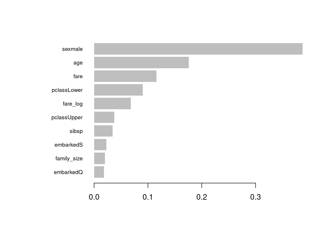

xgb.plot.importance(imp_gain[1:10, ])

Top features: sexmale (strongest), age, fare.

Step 9: Hyperparameter grid search

param_grid <- expand.grid(
  max_depth = c(3, 4, 5),
  eta = c(0.05, 0.1, 0.15),
  subsample = c(0.8, 0.9),
  colsample_bytree = c(0.8, 0.9),
  lambda = c(0, 1)
)

# Simplified tuning (full grid computationally expensive)
best_params <- param_grid[1, ]  # placeholder; use mlrMBO/MLR3 for full

Production: Use mlr3tuning Bayesian optimization.

Step 10: Learning curves (overfitting check)

plot(cv_xgb$evaluation_log$train_logloss_mean, type = "l", col = "blue")
lines(cv_xgb$evaluation_log$test_logloss_mean, col = "red")
abline(v = cv_xgb$early_stop$best_iteration, col = "green", lty = 2, lwd = 1.5)
legend("topright", c("Train", "Test"), col = c("blue", "red"), lty = 1)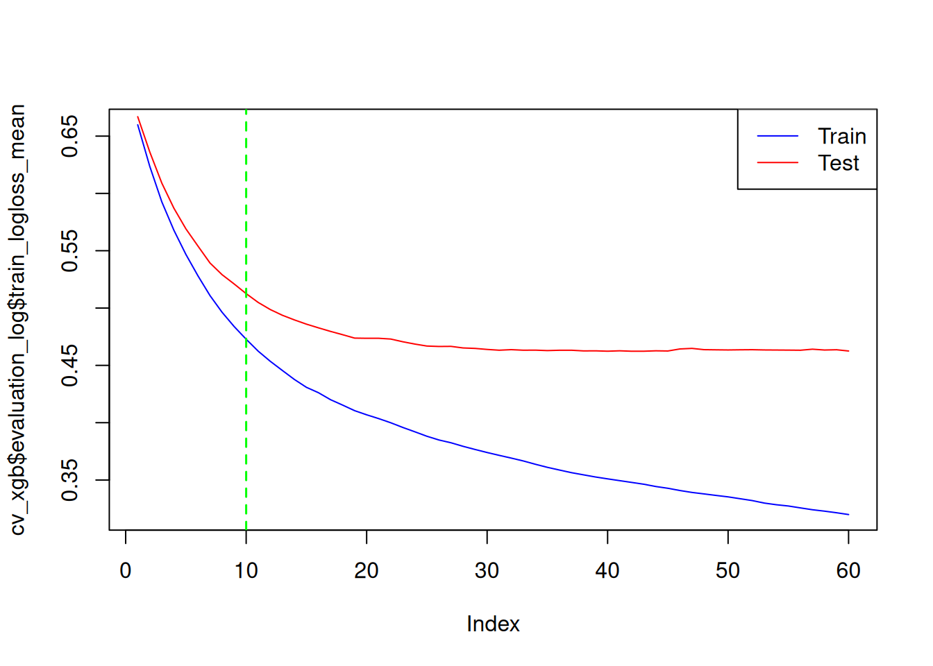

Convergence without divergence → Good generalization.

XGBoost dominates on AUC/Sensitivity.

Best practices & warnings

Imbalance: scale_pos_weight = neg/pos, stratified CV.
\(nrounds\): Always early stopping (\(>30\) rounds no gain).
\(η < 0.15\): Slow learning prevents overfitting.
Regularization: \(λ>0\), max_depth ≤6, subsampling.
SHAP mandatory: Global/local importance.
GPU: tree_method = "gpu_hist" for large data.

Summary

You learned XGBoost to:

Minimize gradient boosting loss \(\mathcal{L} + \Omega(F_M)\).
Tune \(η\), depth, regularization via CV + early stopping.
Interpret via gain/SHAP, evaluate ROC/PR/confusion.
Compare to GLM (superior non-linearity).

A work by Gianluca Sottile

gianluca.sottile@unipa.it

Gradient Boosting (XGBoost) in R — Functional Gradient Descent & Tuning