Hierarchical Clustering in R — Dendrograms, Linkage, Cutting at k, and Comparison with K-means
Hierarchical Clustering
Hierarchical clustering produces a nested sequence of
partitions represented as a dendrogram.
In agglomerative clustering (bottom-up), each observation starts as its
own cluster; clusters are iteratively merged according to a
linkage rule and a distance measure.
Given a dissimilarity \(d(\cdot,\cdot)\), common linkages include:
- Complete: \(d(A,B) = \max_{i \in A, j \in B} d(i,j)\) (tends to compact clusters).
- Average: \(d(A,B) = \frac{1}{|A||B|}\sum_{i \in A, j \in B} d(i,j)\) (balanced).
- Ward: merges that minimize the increase in within-cluster SSE (often strong baseline with Euclidean distance).
In this lesson:
- We build dendrograms with multiple linkages.
- We cut the tree at \(k\).
- We validate clusters with silhouette.
- We compare against K-means using ARI and centroid profiles.
Step 1: Import data (business dataset)
library(readr)
library(dplyr)

local_path <- "raw_data/wholesale_customers.csv"
df_raw <- read_csv(local_path, show_col_types = FALSE)

glimpse(df_raw)
## Rows: 440
## Columns: 8
## $ Channel <dbl> 2, 2, 2, 1, 2, 2, 2, 2, 1, 2, 2, 2, 2, 2, 2, 1, 2, 1,…
## $ Region <dbl> 3, 3, 3, 3, 3, 3, 3, 3, 3, 3, 3, 3, 3, 3, 3, 3, 3, 3,…
## $ Fresh <dbl> 12669, 7057, 6353, 13265, 22615, 9413, 12126, 7579, 5…
## $ Milk <dbl> 9656, 9810, 8808, 1196, 5410, 8259, 3199, 4956, 3648,…
## $ Grocery <dbl> 7561, 9568, 7684, 4221, 7198, 5126, 6975, 9426, 6192,…
## $ Frozen <dbl> 214, 1762, 2405, 6404, 3915, 666, 480, 1669, 425, 115…
## $ Detergents_Paper <dbl> 2674, 3293, 3516, 507, 1777, 1795, 3140, 3321, 1716, …
## $ Delicassen <dbl> 1338, 1776, 7844, 1788, 5185, 1451, 545, 2566, 750, 2…Step 2: Preprocessing (log-transform + scale)
Spending variables are typically right-skewed; a common preprocessing is \(x \leftarrow \log(1+x)\) followed by standardization.
spend_vars <- c("Fresh", "Milk", "Grocery", "Frozen", "Detergents_Paper", "Delicassen")

df <- df_raw |>
  mutate(across(all_of(spend_vars), ~ log1p(.x)))

X <- df |>
  select(all_of(spend_vars)) |>
  mutate(across(everything(), scale)) |>
  as.data.frame()

summary(X)
## Fresh.V1 Milk.V1
## Min. :-4.995530083290 Min. :-3.790608809560000
## 1st Qu.:-0.465406178359 1st Qu.:-0.727333676188000
## Median : 0.214597042110 Median : 0.069236655428600
## Mean : 0.000000000000 Mean :-0.000000000000001
## 3rd Qu.: 0.682916534203 3rd Qu.: 0.702368420716000
## Max. : 1.968421493530 Max. : 2.853333727280000
## Grocery.V1 Frozen.V1
## Min. :-6.347963612920000 Min. :-3.15552594855e+00
## 1st Qu.:-0.690155842996000 1st Qu.:-5.39909432663e-01
## Median : 0.022547740598900 Median : 2.17767536919e-02
## Mean : 0.000000000000001 Mean : 3.00000000000e-16
## 3rd Qu.: 0.748290559456000 3rd Qu.: 6.81065570808e-01
## Max. : 2.695212661690000 Max. : 2.89679595383e+00
## Detergents_Paper.V1 Delicassen.V1
## Min. :-3.16199197814e+00 Min. :-4.084206597810
## 1st Qu.:-7.25228664256e-01 1st Qu.:-0.507568442847
## Median :-5.00371601244e-02 Median : 0.156562527178
## Mean :-1.00000000000e-16 Mean : 0.000000000000
## 3rd Qu.: 8.67386612370e-01 3rd Qu.: 0.646220278446
## Max. : 2.23767100098e+00 Max. : 3.173741392950Step 3: Distances and dendrograms
d <- dist(X, method = "euclidean")

hc_complete <- hclust(d, method = "complete")
hc_average  <- hclust(d, method = "average")
hc_ward     <- hclust(d, method = "ward.D2")

par(mfrow = c(1, 3))
plot(hc_complete, main = "Hierarchical (complete)", cex = 0.6)
plot(hc_average,  main = "Hierarchical (average)",  cex = 0.6)
plot(hc_ward,     main = "Hierarchical (ward.D2)",  cex = 0.6)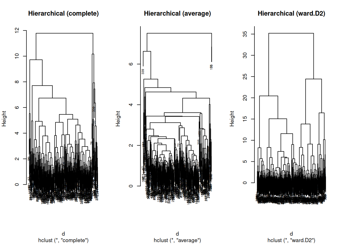
Interpretation guideline:
- Very “chained” dendrograms can indicate poor separation or inappropriate linkage/distance.
- Ward often yields more balanced groups when Euclidean geometry is meaningful.
Step 4: Cutting at k and silhouette validation
We choose a candidate range for \(k\) and compute average silhouette.
library(cluster)
library(ggplot2)

avg_sil <- function(labels, d) {
  s <- silhouette(labels, d)
  mean(s[, 3])
}

k_grid <- 2:12
sil_df <- data.frame(
  k = k_grid,
  sil_complete = NA_real_,
  sil_average  = NA_real_,
  sil_ward     = NA_real_
)

for (i in seq_along(k_grid)) {
  k <- k_grid[i]
  sil_df$sil_complete[i] <- avg_sil(cutree(hc_complete, k = k), d)
  sil_df$sil_average[i]  <- avg_sil(cutree(hc_average,  k = k), d)
  sil_df$sil_ward[i]     <- avg_sil(cutree(hc_ward,     k = k), d)
}

sil_long <- tidyr::pivot_longer(
  sil_df, cols = -k, names_to = "linkage", values_to = "avg_silhouette"
)

ggplot(sil_long, aes(x = k, y = avg_silhouette, color = linkage)) +
  geom_line(linewidth = 1) +
  geom_point(size = 2) +
  theme_minimal() +
  labs(
    title = "Average silhouette for hierarchical clustering",
    x = "Number of clusters (k)",
    y = "Average silhouette"
  )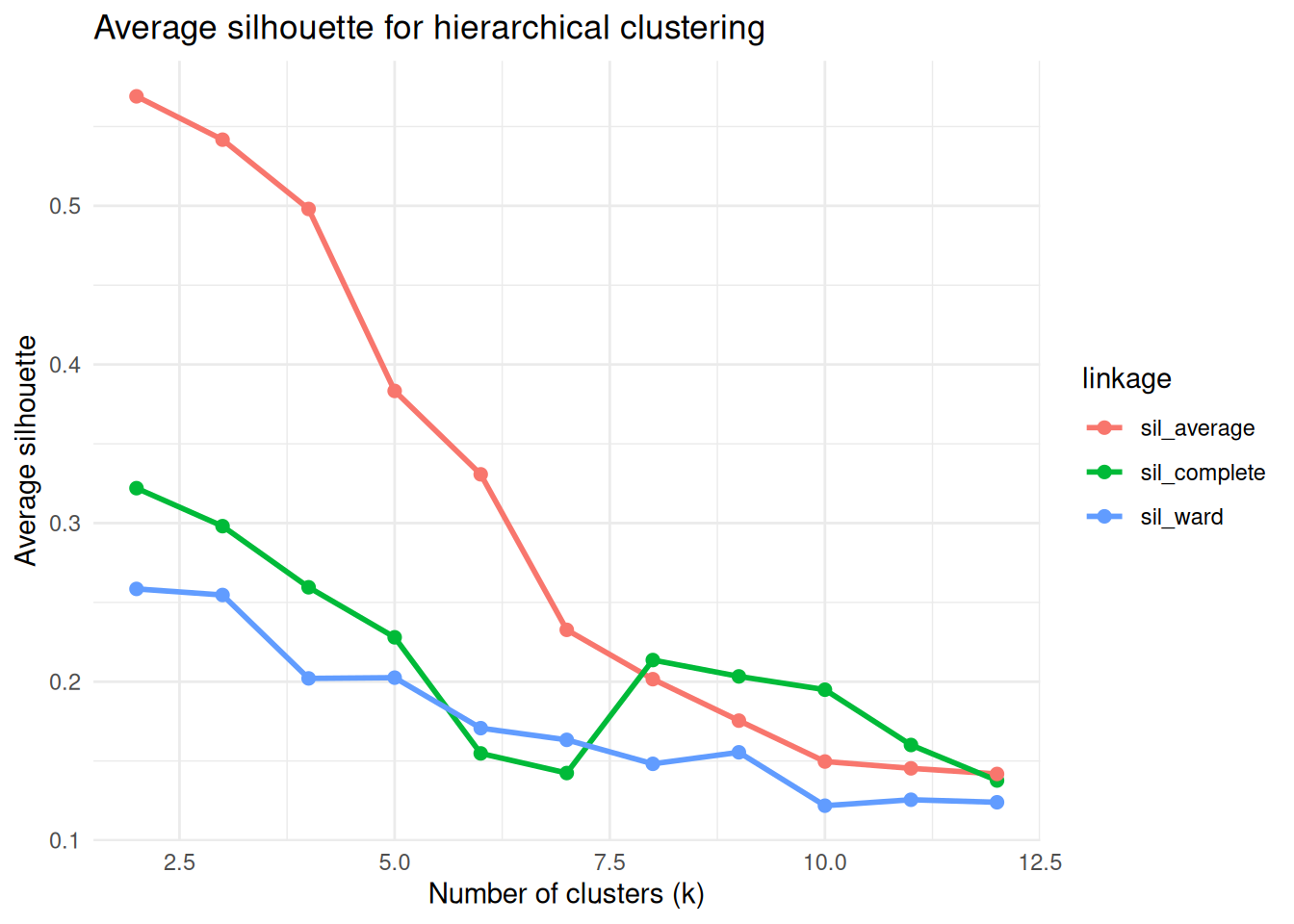
Pick \(k\) where silhouette is reasonably high and the solution is interpretable (avoid excessively tiny clusters unless expected).
Step 5: Final hierarchical solution (example: Ward + chosen k)
## cl_hc
##   1   2
## 178 262
Silhouette plot for the final solution:
sil_obj <- silhouette(cl_hc, d)
plot(sil_obj, border = NA, main = paste("Silhouette plot — Ward, k =", k_final))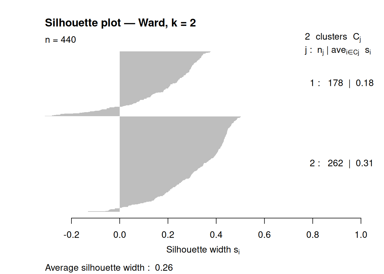
## Silhouette of 440 units in 2 clusters from silhouette.default(x = cl_hc, dist = d) :
##  Cluster sizes and average silhouette widths:
##       178       262
## 0.1753921 0.3149547
## Individual silhouette widths:
##    Min. 1st Qu.  Median    Mean 3rd Qu.    Max.
## -0.3097  0.1784  0.2900  0.2585  0.3921  0.5025
Step 6: Compare with K-means (same k)
K-means minimizes within-cluster SSE: $ (k) = {r=1}^k {i C_r} |x_i - {x}_r|^2 $.
##
##   1   2
## 252 188
Quantitative comparison (Adjusted Rand Index):
## [1] 0.6389459Interpretation:
- ARI close to 0.65: good agreement between partitions.
- Lower ARI: methods capture different structure; investigate cluster shapes, outliers, and linkage choice.
Step 7: Profile clusters (centroid heatmap)
library(tidyr)

centers_hc <- aggregate(X, by = list(cluster = cl_hc), FUN = mean)
centers_long <- centers_hc |>
  pivot_longer(-cluster, names_to = "feature", values_to = "z")

ggplot(centers_long, aes(x = feature, y = factor(cluster), fill = z)) +
  geom_tile(color = "white") +
  scale_fill_gradient2(low = "blue", mid = "white", high = "red", midpoint = 0) +
  theme_minimal() +
  theme(axis.text.x = element_text(angle = 45, hjust = 1)) +
  labs(title = "Hierarchical cluster profiles (z-scores)", x = NULL, y = "Cluster")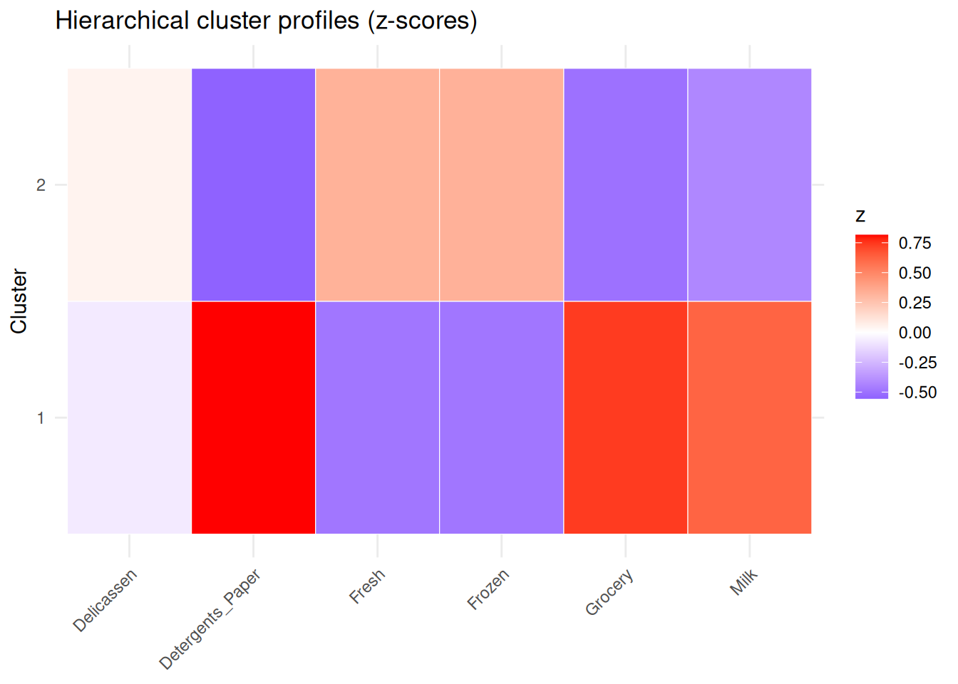
Summary
- Hierarchical clustering provides a dendrogram and supports post-hoc selection of \(k\) by cutting the tree.
- Linkage choice strongly affects results; Ward is often a strong baseline with Euclidean distances.
- Silhouette helps select \(k\) and assess separation.
- Comparing with K-means via ARI and centroid profiles clarifies when the two approaches agree or diverge.
A work by Gianluca Sottile
gianluca.sottile@unipa.it