t-SNE in R — Non-linear Local Structure Visualization
t-SNE (t-Distributed Stochastic Neighbor Embedding)
t-SNE is a non-linear dimensionality reduction technique for high-quality 2D/3D visualizations of high‑dimensional data. It minimizes the KL divergence between high‑D similarities \(P_{ij}\) (Gaussian) and low‑D similarities \(Q_{ij}\) (Student \(t\) distribution):
\[ KL(P \| Q) = \sum_i \sum_j p_{ij} \log \frac{p_{ij}}{q_{ij}} \]
This preserves local neighborhoods (close points
stay close) better than linear methods like PCA, at the expense of
global structure. t-SNE is stochastic and
iterative; key parameter is perplexity (\(5 \leq perpl \leq 50\)), balancing
local/global focus.
In this lesson we apply t-SNE to iris, comparing to PCA,
and explore parameter sensitivity.
Step 1: Data preparation
data("iris")
iris_num <- iris |>
  dplyr::select(where(is.numeric)) |>
  scale(center = TRUE, scale = TRUE)  # standardize like PCA

glimpse(iris_num)
## num [1:150, 1:4] -0.898 -1.139 -1.381 -1.501 -1.018 ...
## - attr(*, "dimnames")=List of 2
## ..$ : NULL
## ..$ : chr [1:4] "Sepal.Length" "Sepal.Width" "Petal.Length" "Petal.Width"
## - attr(*, "scaled:center")= Named num [1:4] 5.84 3.06 3.76 1.2
## ..- attr(*, "names")= chr [1:4] "Sepal.Length" "Sepal.Width" "Petal.Length" "Petal.Width"
## - attr(*, "scaled:scale")= Named num [1:4] 0.828 0.436 1.765 0.762
## ..- attr(*, "names")= chr [1:4] "Sepal.Length" "Sepal.Width" "Petal.Length" "Petal.Width"Standardization ensures features contribute equally, as in PCA.
Step 2: Compute t-SNE embedding
library(Rtsne)

set.seed(123)
tsne_iris <- Rtsne(
  X = iris_num,
  dims = 2,
  perplexity = 30,        # effective neighbors per point
  theta = 0.0,            # exact computation (no approx)
  check_duplicates = FALSE,
  verbose = TRUE
)
## Performing PCA
## Read the 150 x 4 data matrix successfully!
## OpenMP is working. 1 threads.
## Using no_dims = 2, perplexity = 30.000000, and theta = 0.000000
## Computing input similarities...
## Symmetrizing...
## Done in 0.00 seconds!
## Learning embedding...
## Iteration 50: error is 48.262304 (50 iterations in 0.01 seconds)
## Iteration 100: error is 46.793373 (50 iterations in 0.01 seconds)
## Iteration 150: error is 46.484400 (50 iterations in 0.01 seconds)
## Iteration 200: error is 46.689979 (50 iterations in 0.01 seconds)
## Iteration 250: error is 44.901001 (50 iterations in 0.01 seconds)
## Iteration 300: error is 0.393504 (50 iterations in 0.01 seconds)
## Iteration 350: error is 0.170058 (50 iterations in 0.01 seconds)
## Iteration 400: error is 0.162646 (50 iterations in 0.01 seconds)
## Iteration 450: error is 0.160359 (50 iterations in 0.01 seconds)
## Iteration 500: error is 0.159208 (50 iterations in 0.01 seconds)
## Iteration 550: error is 0.158620 (50 iterations in 0.01 seconds)
## Iteration 600: error is 0.158261 (50 iterations in 0.01 seconds)
## Iteration 650: error is 0.158016 (50 iterations in 0.01 seconds)
## Iteration 700: error is 0.157838 (50 iterations in 0.01 seconds)
## Iteration 750: error is 0.157705 (50 iterations in 0.01 seconds)
## Iteration 800: error is 0.157606 (50 iterations in 0.01 seconds)
## Iteration 850: error is 0.157528 (50 iterations in 0.01 seconds)
## Iteration 900: error is 0.157464 (50 iterations in 0.01 seconds)
## Iteration 950: error is 0.157414 (50 iterations in 0.01 seconds)
## Iteration 1000: error is 0.157372 (50 iterations in 0.01 seconds)
## Fitting performed in 0.13 seconds.## List of 14
## $ N : int 150
## $ Y : num [1:150, 1:2] 22.1 18.2 19.4 18.7 22.6 ...
## $ costs : num [1:150] -4.72e-04 -9.07e-05 -3.51e-04 -5.78e-04 -1.30e-04 ...
## $ itercosts : num [1:20] 48.3 46.8 46.5 46.7 44.9 ...
## $ origD : int 4
## $ perplexity : num 30
## $ theta : num 0
## $ max_iter : num 1000
## $ stop_lying_iter : int 250
## $ mom_switch_iter : int 250
## $ momentum : num 0.5
## $ final_momentum : num 0.8
## $ eta : num 200
## $ exaggeration_factor: num 12
## - attr(*, "class")= chr [1:2] "Rtsne" "list"## [,1] [,2]
## [1,] 22.07374 -4.453237
## [2,] 18.20858 -4.357915
## [3,] 19.38024 -3.644687Key outputs:
Y: \(150 \times 2\) embedding coordinates.
N: Number of objects.
perplexity: Used value (printed during computation).
Step 3: Visualization and cluster separation
library(ggplot2)

tsne_df <- data.frame(
  tsne1 = tsne_iris$Y[, 1],
  tsne2 = tsne_iris$Y[, 2],
  Species = iris$Species
)

ggplot(tsne_df, aes(x = tsne1, y = tsne2, color = Species)) +
  geom_point(size = 3, alpha = 0.8) +
  labs(
    title = "t-SNE Embedding — Iris Dataset",
    subtitle = "Perplexity = 30 | Three species clearly separated",
    x = "t-SNE Dimension 1",
    y = "t-SNE Dimension 2"
  ) +
  theme_minimal() +
  theme(legend.position = "bottom")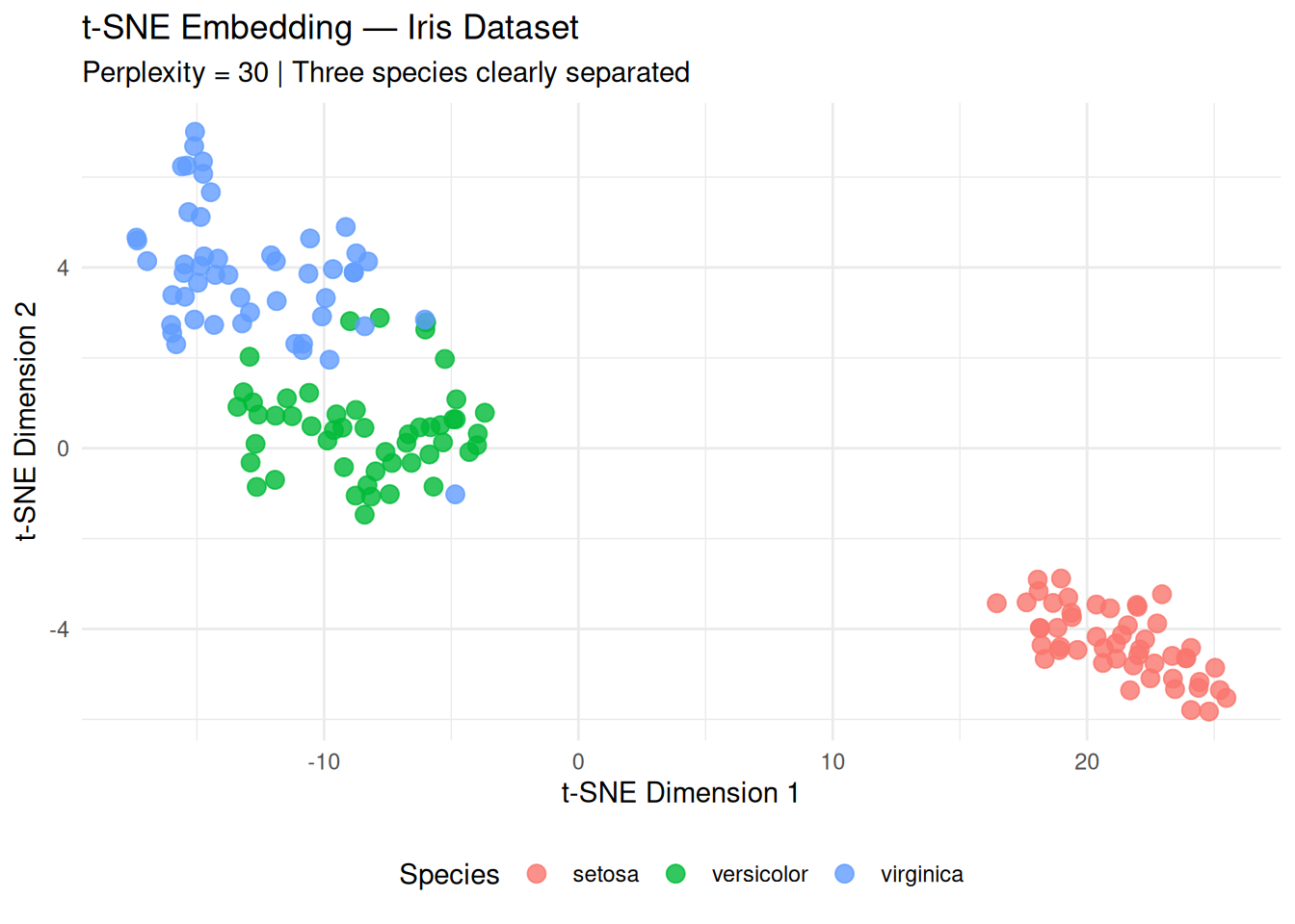
Interpretation:
- setosa perfectly separated (bottom‑left).
- versicolor and virginica form
adjacent but distinct clusters (local structure preserved).
- Unlike PCA scores (linear), t-SNE reveals non-linear manifolds.
Step 4: Parameter sensitivity — perplexity effect
# Compare perplexity 5 (local) vs 50 (global)
set.seed(123)
tsne_low  <- Rtsne(iris_num, check_duplicates = FALSE, dims = 2, perplexity = 5,  verbose = FALSE)$Y
tsne_high <- Rtsne(iris_num, check_duplicates = FALSE, dims = 2, perplexity = 40, verbose = FALSE)$Y

par(mfrow = c(1, 2))
plot(tsne_low,  col = as.numeric(iris$Species), pch = 19, main = "Perplexity = 5 (local)")
plot(tsne_high, col = as.numeric(iris$Species), pch = 19, main = "Perplexity = 40 (global)")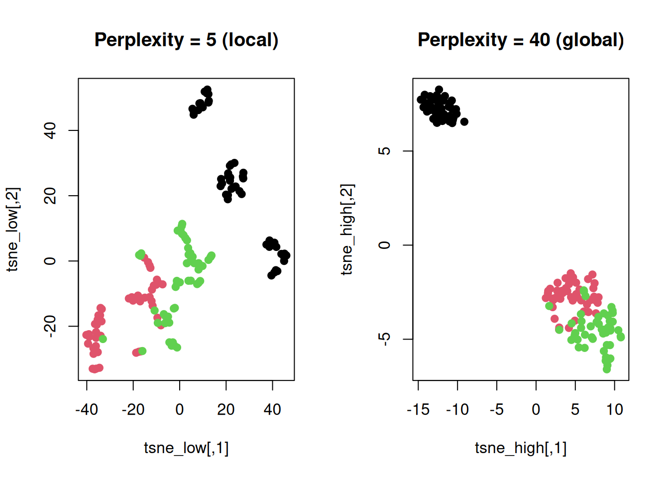
Low perplexity: Tight clusters, poor global
view.
High perplexity: Better global layout, looser
clusters.
Step 5: Validation — cluster purity vs PCA
# Silhouette score (higher = better separation)
library(cluster)
sil_tsne <- silhouette(as.numeric(iris$Species), dist(tsne_iris$Y))
mean(sil_tsne[, 3])  # average silhouette width
## [1] 0.5394205# Compare to PCA
pca_iris <- prcomp(iris_num)
sil_pca <- silhouette(as.numeric(iris$Species), dist(pca_iris$x[, 1:2]))
cat("t-SNE silhouette:", round(mean(sil_tsne[, 3]), 3), "\n")## t-SNE silhouette: 0.539## PCA silhouette: 0.401t-SNE often shows higher silhouette than PCA due to local optimization.
Step 6: High-D embedding (3D for animation)
Warnings and best practices
- Stochastic: Always set
seed.
- Not for modeling: Distances in t-SNE space
meaningless; use only for
exploration/visualization.
- Scales poorly (> 10k points: use UMAP).
- Perplexity rule: \(perpl \approx 3\%\) of \[n\] (here \(30 \approx 20\%\) fine).
Summary
You learned t-SNE with Rtsne() to:
- Compute non-linear embeddings minimizing \(KL(P \| Q)\).
- Tune
perplexityand interpret local cluster structure.
- Compare quantitatively to PCA via silhouette scores.
t-SNE excels at revealing hidden clusters in exploratory analysis.
A work by Gianluca Sottile
gianluca.sottile@unipa.it