UMAP in R — Scalable Non-linear Embedding
UMAP (Uniform Manifold Approximation and Projection)
UMAP constructs a fuzzy topological representation of the high‑D data manifold using weighted k‑nearest neighbor graphs, then optimizes low‑D coordinates minimizing cross-entropy loss:
\[ CE = \sum_{ij} \left[ v_{ij} \log \frac{v_{ij}}{u_{ij}} + (1 - v_{ij}) \log \frac{1 - v_{ij}}{1 - u_{ij}} \right] \]
where \(v_{ij}\) (high‑D) and \(u_{ij}\) (low‑D) are fuzzy simplicial set probabilities. UMAP balances local structure (\(n_neighbors\)) and global layout (\(min_dist\)), outperforming t-SNE in speed and scalability while preserving both.[1][2]
In this lesson we apply UMAP to iris, compare with
t-SNE/PCA, and tune key parameters.
Step 1: Data preparation
data("iris")
iris_num <- iris |>
  dplyr::select(where(is.numeric)) |>
  scale(center = TRUE, scale = TRUE)  # standardize

glimpse(iris_num)
## num [1:150, 1:4] -0.898 -1.139 -1.381 -1.501 -1.018 ...
## - attr(*, "dimnames")=List of 2
## ..$ : NULL
## ..$ : chr [1:4] "Sepal.Length" "Sepal.Width" "Petal.Length" "Petal.Width"
## - attr(*, "scaled:center")= Named num [1:4] 5.84 3.06 3.76 1.2
## ..- attr(*, "names")= chr [1:4] "Sepal.Length" "Sepal.Width" "Petal.Length" "Petal.Width"
## - attr(*, "scaled:scale")= Named num [1:4] 0.828 0.436 1.765 0.762
## ..- attr(*, "names")= chr [1:4] "Sepal.Length" "Sepal.Width" "Petal.Length" "Petal.Width"Step 2: Baseline UMAP embedding
library(uwot)

set.seed(123)
umap_iris <- umap(
  X = iris_num,
  n_neighbors = 15,      # local neighborhood size (~ perplexity)
  min_dist = 0.1,        # min distance in low-D (cluster tightness)
  n_components = 2,
  metric = "euclidean",
  n_threads = 0,         # auto-detect cores
  verbose = TRUE
)

dim(umap_iris)
## [1] 150 2## [,1] [,2]
## [1,] 10.154459 1.840331
## [2,] 9.260841 4.203367
## [3,] 8.893306 3.416821Key parameters:
n_neighbors: \(k\) in kNN graph (\(5 \leq k \leq \min(15, n/3)\)); low = local focus, high = global.
min_dist: Separation in low-D (\(0.001–0.5\)); low = tight clusters.
- Deterministic given seed (unlike t-SNE).
Step 3: Visualization
library(ggplot2)

umap_df <- data.frame(
  umap1 = umap_iris[, 1],
  umap2 = umap_iris[, 2],
  Species = iris$Species
)

ggplot(umap_df, aes(x = umap1, y = umap2, color = Species)) +
  geom_point(size = 3, alpha = 0.8) +
  labs(
    title = "UMAP Embedding — Iris Dataset",
    subtitle = "n_neighbors=15, min_dist=0.1 | Local + global structure preserved",
    x = "UMAP Dimension 1",
    y = "UMAP Dimension 2"
  ) +
  theme_minimal() +
  theme(legend.position = "bottom")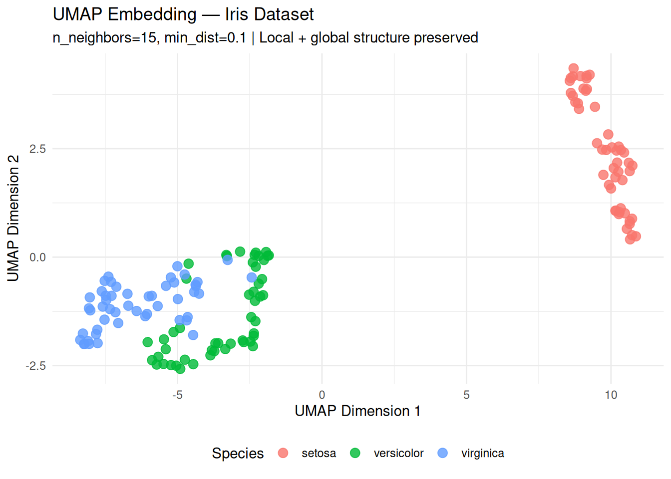
Interpretation:
- setosa clearly separated (global structure).
- versicolor/virginica tight yet
distinct (local structure).
- Superior to t-SNE in global distances preservation.
Step 4: Parameter sensitivity — n_neighbors effect
# Low n_neighbors (local focus)
umap_local <- umap(iris_num, n_neighbors = 5, min_dist = 0.1, n_components = 2)

# High n_neighbors (global focus)
umap_global <- umap(iris_num, n_neighbors = 40, min_dist = 0.1, n_components = 2)

par(mfrow = c(1, 2))
plot(umap_local, col = as.numeric(iris$Species), pch = 19,
     main = "n_neighbors = 5 (local)")
plot(umap_global, col = as.numeric(iris$Species), pch = 19,
     main = "n_neighbors = 40 (global)")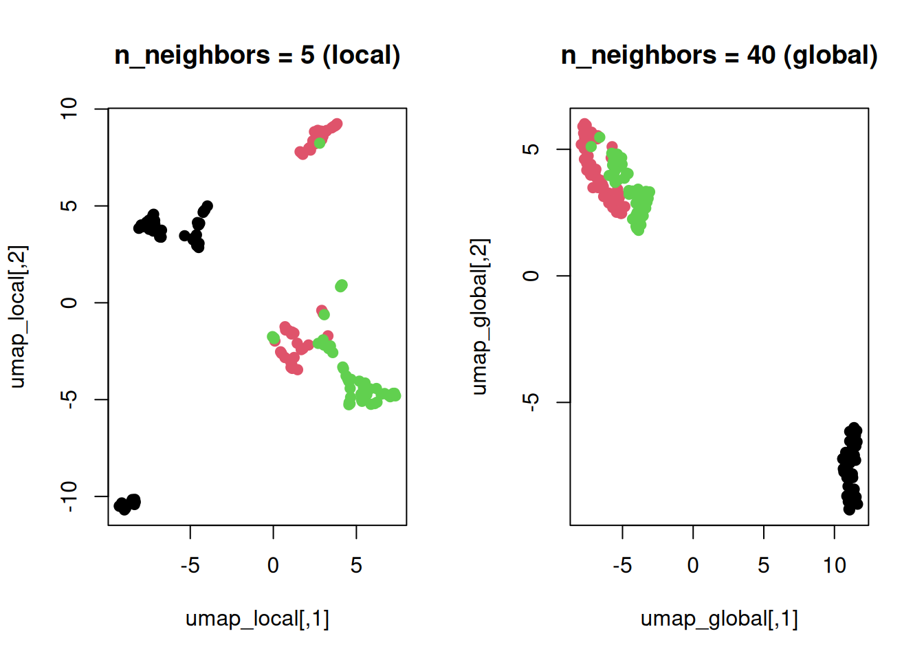
Low \(k\): Tight
clusters, fragmented global view.
High \(k\): Cohesive
layout, looser local structure.
Step 5: Quantitative validation — silhouette & comparison
library(cluster)

# UMAP silhouette
sil_umap <- silhouette(as.numeric(iris$Species), dist(umap_iris))
mean(sil_umap[, 3])
## [1] 0.5188071# Compare: PCA, t-SNE (from Lesson 33)
pca_iris <- prcomp(iris_num)
sil_pca <- silhouette(as.numeric(iris$Species), dist(pca_iris$x[, 1:2]))
cat("UMAP silhouette:", round(mean(sil_umap[, 3]), 3), "\n")## UMAP silhouette: 0.519## PCA silhouette: 0.401UMAP typically achieves high silhouette (good separation) with better global preservation than t-SNE.
Step 6: UMAP as features (supervised use case)
# Use UMAP coordinates as input to kNN
set.seed(123)
n <- nrow(umap_iris)
train_idx <- sample(n, floor(0.7 * n))

umap_train <- umap_iris[train_idx, ]
umap_test  <- umap_iris[-train_idx, ]
species_train <- iris$Species[train_idx]
species_test  <- iris$Species[-train_idx]

library(caret)
knn_umap <- train(
  x = data.frame(umap_train),
  y = species_train,
  method = "knn",
  trControl = trainControl(method = "cv", number = 5)
)

pred_umap <- predict(knn_umap, newdata = data.frame(umap_test))
confusionMatrix(pred_umap, species_test)
## Confusion Matrix and Statistics
##
## Reference
## Prediction setosa versicolor virginica
## setosa 14 0 0
## versicolor 0 17 0
## virginica 0 1 13
##
## Overall Statistics
##
## Accuracy : 0.9778
## 95% CI : (0.8823, 0.9994)
## No Information Rate : 0.4
## P-Value [Acc > NIR] : < 2.2e-16
##
## Kappa : 0.9664
##
## Mcnemar's Test P-Value : NA
##
## Statistics by Class:
##
## Class: setosa Class: versicolor Class: virginica
## Sensitivity 1.0000 0.9444 1.0000
## Specificity 1.0000 1.0000 0.9688
## Pos Pred Value 1.0000 1.0000 0.9286
## Neg Pred Value 1.0000 0.9643 1.0000
## Prevalence 0.3111 0.4000 0.2889
## Detection Rate 0.3111 0.3778 0.2889
## Detection Prevalence 0.3111 0.3778 0.3111
## Balanced Accuracy 1.0000 0.9722 0.9844UMAP embeddings work as effective low‑D features for classification (better than raw high‑D in some cases).
Best practices
- \(n_neighbors \approx
15\) (default good start); scale with \(\sqrt{n}\).
min_dist = 0.1for publication plots.
- Scales to millions of points (GPU support
available).
- Safe for modeling: Unlike t-SNE, preserves
meaningful distances.
- Metric choice: Euclidean default; try
"cosine"for sparse/text data.
Summary
You learned UMAP with uwot::umap() to:
- Build scalable non-linear embeddings via fuzzy
simplicial sets.
- Tune
n_neighbors/min_distand validate with silhouette scores.
- Use embeddings as model features (unlike pure visualization methods).
UMAP is state-of-the-art for both exploration and production pipelines.
A work by Gianluca Sottile
gianluca.sottile@unipa.it