Model-based clustering (Gaussian Mixture Models)

Model-based clustering assumes data arise from a mixture distribution: \(p(x) = \sum_{g=1}^G \pi_g \, \phi(x \mid \mu_g, \Sigma_g)\), where \(\pi_g \ge 0\) and \(\sum_g \pi_g = 1\).

Key properties:

Soft assignments via posterior probabilities: \(\tau_{ig} = P(z_i=g \mid x_i)\).
Clusters can be elliptical (through \(\Sigma_g\)), unlike K-means which is inherently spherical in Euclidean space.
The number of components \(G\) can be selected using information criteria (commonly BIC).

In this lesson:

Fit a GMM with automatic model selection.
Inspect soft assignments (uncertainty).
Compare with K-means.

Step 1: Import + preprocessing

library(readr)
library(dplyr)

local_path <- "raw_data/wholesale_customers.csv"
df_raw <- read_csv(local_path, show_col_types = FALSE)

spend_vars <- c("Fresh", "Milk", "Grocery", "Frozen", "Detergents_Paper", "Delicassen")

X <- df_raw |>
  mutate(across(all_of(spend_vars), ~ log1p(.x))) |>
  select(all_of(spend_vars)) |>
  mutate(across(everything(), scale)) |>
  as.matrix()

Step 2: Fit model-based clustering and select G by BIC

# install.packages("mclust")  # if needed
library(mclust)

set.seed(123)
fit <- Mclust(X, G = 1:12, verbose = FALSE)

fit

## 'Mclust' model object: (VVE,5) 
## 
## Available components: 
##  [1] "call"           "data"           "modelName"      "n"             
##  [5] "d"              "G"              "BIC"            "loglik"        
##  [9] "df"             "bic"            "icl"            "hypvol"        
## [13] "parameters"     "z"              "classification" "uncertainty"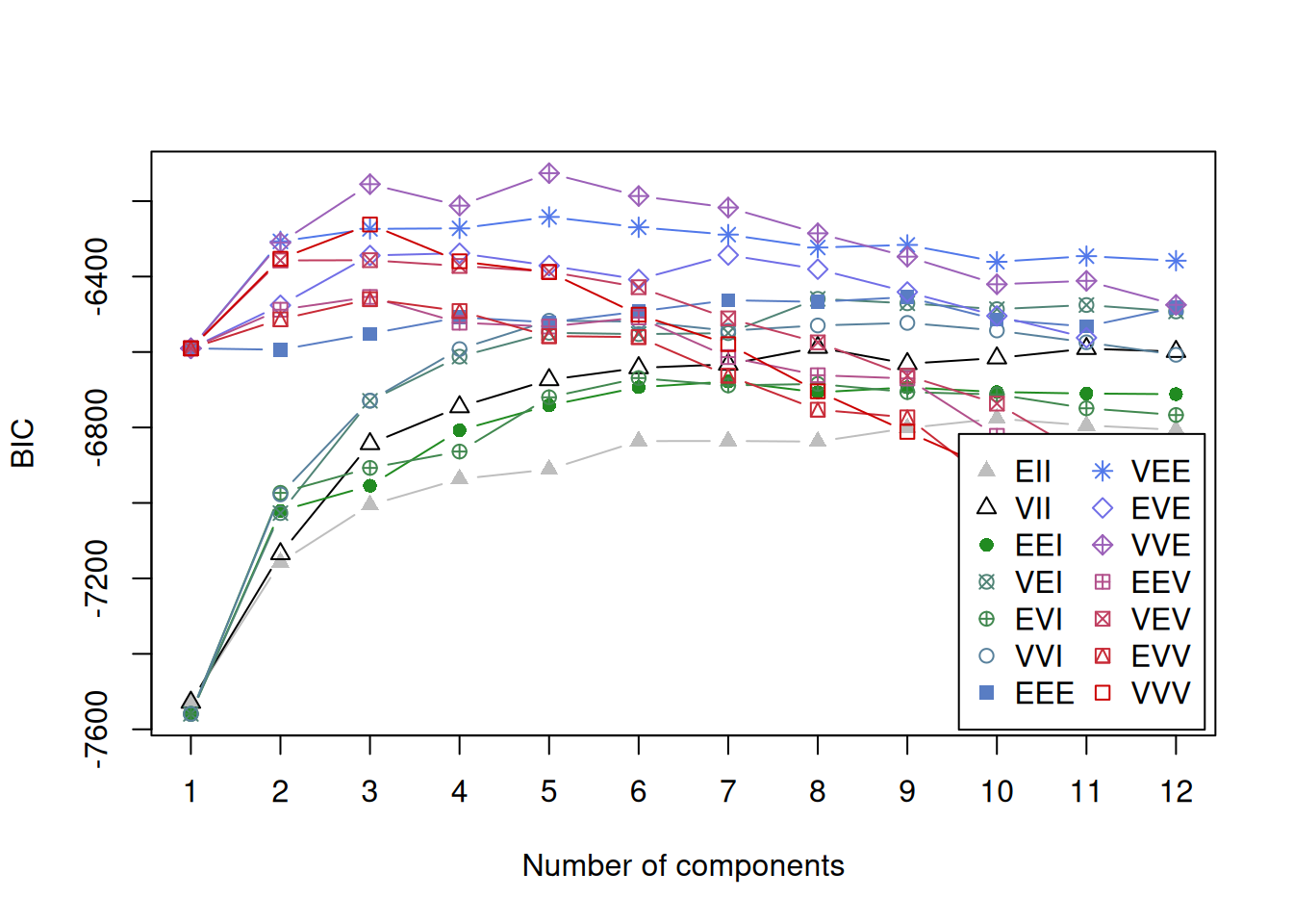

plot(fit, what = "BIC")

Commentary:

If the BIC curve has a clear maximum, the selected \(G\) is usually stable.
If BIC is flat across many \(G\), clustering structure may be weak or sensitive to preprocessing.

Step 3: Hard vs soft clustering outputs

cl <- fit$classification          # hard labels
prob <- fit$z                     # posterior probabilities (n x G)
uncert <- 1 - apply(prob, 1, max) # simple uncertainty measure

table(cl)

## cl
##   1   2   3   4   5 
##  51 101 155  81  52

summary(uncert)

##    Min. 1st Qu.  Median    Mean 3rd Qu.    Max. 
## 0.00000 0.01345 0.04573 0.11402 0.16097 0.60119

High uncertainty points indicate observations not clearly explained by any single component.

Step 4: Visualization (PCA + uncertainty)

library(ggplot2)

pc <- prcomp(X)
plot_df <- data.frame(
  PC1 = pc$x[, 1],
  PC2 = pc$x[, 2],
  cluster = factor(cl),
  uncertainty = uncert
)

ggplot(plot_df, aes(PC1, PC2, color = cluster)) +
  geom_point(aes(alpha = 1 - uncertainty), size = 2) +
  theme_minimal() +
  labs(
    title = "Model-based clustering (GMM) — PCA projection",
    subtitle = "Point transparency reflects assignment certainty",
    x = "PC1", y = "PC2"
  )

Step 5: Compare with K-means (same number of clusters)

set.seed(123)
km <- kmeans(X, centers = length(unique(cl)), nstart = 50)

ari <- adjustedRandIndex(cl, km$cluster)
ari

## [1] 0.3911639

Interpretation:

If ARI is high, both methods recover similar structure.
If ARI is lower, investigate covariance shapes: GMM can fit ellipses; K-means cannot.

Step 6: Cluster profiling

df_prof <- as.data.frame(X)
df_prof$cluster <- factor(cl)

profiles <- df_prof |>
  group_by(cluster) |>
  summarize(across(where(is.numeric), mean), .groups = "drop")

profiles

cluster	Fresh	Milk	Grocery	Frozen	Detergents_Paper	Delicassen
1	-1.0655120	0.7999948	1.0069265	-1.2232358	1.1661900	-0.2222957
2	0.1712266	0.8216657	0.8652300	-0.0062327	1.0215707	0.4978113
3	0.5462568	-0.5670315	-0.5730281	0.6567221	-0.5986691	0.1313179
4	-0.0650259	-0.1181184	-0.2940579	-0.2959572	-0.2604843	-0.1358719
5	-0.8145286	-0.5063557	-0.5019892	-0.2847088	-0.9377190	-0.9286635

For business communication, it is often preferable to profile clusters on original-scale variables (before scaling/log), and report relative differences.

Summary

Model-based clustering provides a probabilistic framework with soft assignments.
It naturally supports elliptical clusters and explicit uncertainty quantification.
BIC-based selection helps choose the number of components.
Comparing GMM vs K-means clarifies whether “spherical” clustering is too restrictive.

A work by Gianluca Sottile

gianluca.sottile@unipa.it

Model-based Clustering in R — Gaussian Mixtures, Soft Assignments, and Component Selection