Ridge & Lasso Regression (Penalized OLS)

Why penalization?

OLS estimates can become unstable when:

predictors are highly correlated (multicollinearity),
the number of predictors is large relative to the sample size,
you want a model that generalizes better (lower variance) and/or performs variable selection.

Penalized regression adds a constraint/penalty to shrink coefficients toward zero, trading a bit of bias for lower variance.

Theory: Ridge, Lasso, Elastic Net

Assume a linear model \(y = X\beta + \epsilon\) with \(X \in \mathbb{R}^{n \times p}\). The OLS objective minimizes RSS: \[ \min_{\beta_0,\beta}\ \frac{1}{2n}\sum_{i=1}^n (y_i - \beta_0 - x_i^T\beta)^2 \]

Ridge (L2 penalty)

\[ \min_{\beta_0,\beta}\ \frac{1}{2n}\sum_{i=1}^n (y_i - \beta_0 - x_i^T\beta)^2\ +\ \lambda \sum_{j=1}^p \beta_j^2 \]

Shrinks coefficients smoothly.
Typically does not set coefficients exactly to zero (no hard feature selection).
Very useful under multicollinearity.

Lasso (L1 penalty)

\[ \min_{\beta_0,\beta}\ \frac{1}{2n}\sum_{i=1}^n (y_i - \beta_0 - x_i^T\beta)^2\ +\ \lambda \sum_{j=1}^p |\beta_j| \]

Encourages sparsity: some \(\hat\beta_j = 0\).
Performs variable selection (often easier interpretation).

Elastic Net (mix L1 + L2)

Elastic Net combines both: \[ \min_{\beta_0,\beta}\ \frac{1}{2n}\|y-\beta_0\mathbf{1}-X\beta\|_2^2 \ +\ \lambda\left[(1-\alpha)\frac{1}{2}\|\beta\|_2^2 + \alpha\|\beta\|_1\right] \] with \(0 \le \alpha \le 1\):

\(\alpha = 0\) → ridge
\(\alpha = 1\) → lasso
\(0<\alpha<1\) → elastic net

Hyperparameter intuition

\(\lambda = 0\): no penalization (≈ OLS).
\(\lambda \uparrow\): stronger shrinkage; lasso sets more coefficients to zero.
\(\alpha\): controls sparsity vs stability.

Practice in R with glmnet

Key points:

glmnet expects a numeric matrix x (use model.matrix() for factors).
Use cross-validation to select \(\lambda\) via cv.glmnet().
Common choices:
- lambda.min: minimizes CV error.
- lambda.1se: simplest model within 1 standard error (more regularization; often more robust).

Example: Ridge vs Lasso on mtcars (Gaussian regression)

We predict mpg using a mix of numeric and categorical features.

Step 1: Data preparation (design matrix)

library(dplyr)

df <- mtcars |>
  mutate(
    cyl = factor(cyl),
    am  = factor(am, labels = c("auto", "manual")),
    vs  = factor(vs)
  )

# Model matrix: adds intercept column by default; glmnet handles intercept separately,
# so we remove it with "-1" here and let glmnet fit intercept = TRUE.
X <- model.matrix(mpg ~ . - 1, data = df)
y <- df$mpg

dim(X)

## [1] 32 12

head(X[, 1:6])

##                   cyl4 cyl6 cyl8 disp  hp drat
## Mazda RX4            0    1    0  160 110 3.90
## Mazda RX4 Wag        0    1    0  160 110 3.90
## Datsun 710           1    0    0  108  93 3.85
## Hornet 4 Drive       0    1    0  258 110 3.08
## Hornet Sportabout    0    0    1  360 175 3.15
## Valiant              0    1    0  225 105 2.76

Step 2: Train/test split

set.seed(123)
n <- nrow(X)
idx_train <- sample.int(n, size = floor(0.75 * n))

X_train <- X[idx_train, , drop = FALSE]
y_train <- y[idx_train]

X_test <- X[-idx_train, , drop = FALSE]
y_test <- y[-idx_train]

Step 3: Baseline OLS (for comparison)

train_ols <- data.frame(mpg = y_train, X_train)
test_ols  <- data.frame(mpg = y_test,  X_test)

fit_ols <- lm(mpg ~ ., data = train_ols)
summary(fit_ols)

## 
## Call:
## lm(formula = mpg ~ ., data = train_ols)
## 
## Residuals:
##     Min      1Q  Median      3Q     Max 
## -3.7677 -1.3928 -0.0578  0.7350  4.6582 
## 
## Coefficients: (1 not defined because of singularities)
##             Estimate Std. Error t value Pr(>|t|)  
## (Intercept) 16.57753   19.19814   0.863   0.4048  
## cyl4         2.46724    6.70666   0.368   0.7194  
## cyl6        -0.20269    4.81932  -0.042   0.9671  
## cyl8              NA         NA      NA       NA  
## disp         0.02219    0.02786   0.797   0.4411  
## hp          -0.03423    0.04199  -0.815   0.4308  
## drat        -0.12025    2.31432  -0.052   0.9594  
## wt          -4.53231    2.54011  -1.784   0.0997 .
## qsec         0.75808    0.95328   0.795   0.4419  
## vs1          1.53834    2.93413   0.524   0.6096  
## ammanual     2.47468    2.99684   0.826   0.4251  
## gear         0.12976    2.20021   0.059   0.9539  
## carb         0.64798    1.23947   0.523   0.6106  
## ---
## Signif. codes:  0 '***' 0.001 '**' 0.01 '*' 0.05 '.' 0.1 ' ' 1
## 
## Residual standard error: 3.033 on 12 degrees of freedom
## Multiple R-squared:  0.8818, Adjusted R-squared:  0.7734 
## F-statistic: 8.138 on 11 and 12 DF,  p-value: 0.0005336

pred_ols <- predict(fit_ols, newdata = test_ols)
rmse <- function(y, yhat) sqrt(mean((y - yhat)^2))

rmse_ols <- rmse(y_test, pred_ols)
rmse_ols

## [1] 2.1292

Step 4: Ridge regression (alpha = 0) with CV

# install.packages("glmnet")  # if needed
library(glmnet)

set.seed(123)
cv_ridge <- cv.glmnet(
  x = X_train,
  y = y_train,
  alpha = 0,            # ridge
  nfolds = 10,          # default is 10
  standardize = TRUE
)

plot(cv_ridge)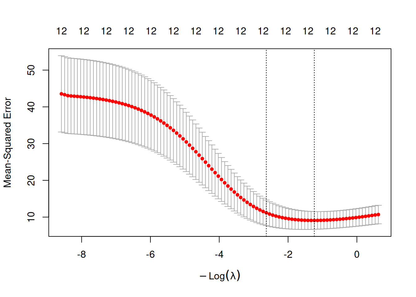

cv_ridge$lambda.min

## [1] 3.444694

cv_ridge$lambda.1se

## [1] 13.90629

Fit ridge at selected lambda and evaluate:

pred_ridge_min <- predict(cv_ridge, newx = X_test, s = "lambda.min")
pred_ridge_1se <- predict(cv_ridge, newx = X_test, s = "lambda.1se")

rmse_ridge_min <- rmse(y_test, pred_ridge_min)
rmse_ridge_1se <- rmse(y_test, pred_ridge_1se)

c(rmse_ols = rmse_ols, rmse_ridge_min = rmse_ridge_min, rmse_ridge_1se = rmse_ridge_1se)

##       rmse_ols rmse_ridge_min rmse_ridge_1se 
##       2.129200       2.055639       2.218518

Inspect coefficients:

coef(cv_ridge, s = "lambda.min")[1:10, , drop = FALSE]

## 10 x 1 sparse Matrix of class "dgCMatrix"
##               lambda.min
## (Intercept) 20.049804674
## cyl4         1.509365191
## cyl6        -0.715565529
## cyl8        -1.064064671
## disp        -0.005891425
## hp          -0.010170279
## drat         0.913128419
## wt          -1.233903891
## qsec         0.153282689
## vs1          1.011905504

Step 5: Lasso regression (alpha = 1) with CV

set.seed(123)
cv_lasso <- cv.glmnet(
  x = X_train,
  y = y_train,
  alpha = 1,            # lasso
  nfolds = 10,
  standardize = TRUE
)

plot(cv_lasso)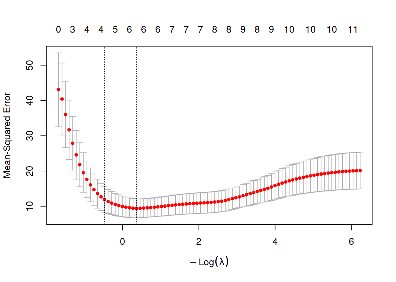

cv_lasso$lambda.min

## [1] 0.6921193

cv_lasso$lambda.1se

## [1] 1.598885

Evaluate and compare:

pred_lasso_min <- predict(cv_lasso, newx = X_test, s = "lambda.min")
pred_lasso_1se <- predict(cv_lasso, newx = X_test, s = "lambda.1se")

rmse_lasso_min <- rmse(y_test, pred_lasso_min)
rmse_lasso_1se <- rmse(y_test, pred_lasso_1se)

c(
  rmse_ols = rmse_ols,
  rmse_lasso_min = rmse_lasso_min,
  rmse_lasso_1se = rmse_lasso_1se
)

##       rmse_ols rmse_lasso_min rmse_lasso_1se 
##       2.129200       2.060473       2.171117

Check sparsity (number of non-zero coefficients):

b_lasso_min <- coef(cv_lasso, s = "lambda.min")
nnz <- sum(b_lasso_min != 0)
nnz

## [1] 6

List selected predictors:

selected <- rownames(b_lasso_min)[as.vector(b_lasso_min != 0)]
selected

## [1] "(Intercept)" "cyl4"        "cyl8"        "hp"          "wt"         
## [6] "vs1"

Step 6: Coefficient paths (optional)

fit_lasso_path <- glmnet(X_train, y_train, alpha = 1, standardize = TRUE)
plot(fit_lasso_path, xvar = "lambda", label = TRUE, main = "Lasso coefficient paths")
abline(v = -log(cv_lasso$lambda.min), lty = 2, col = "red")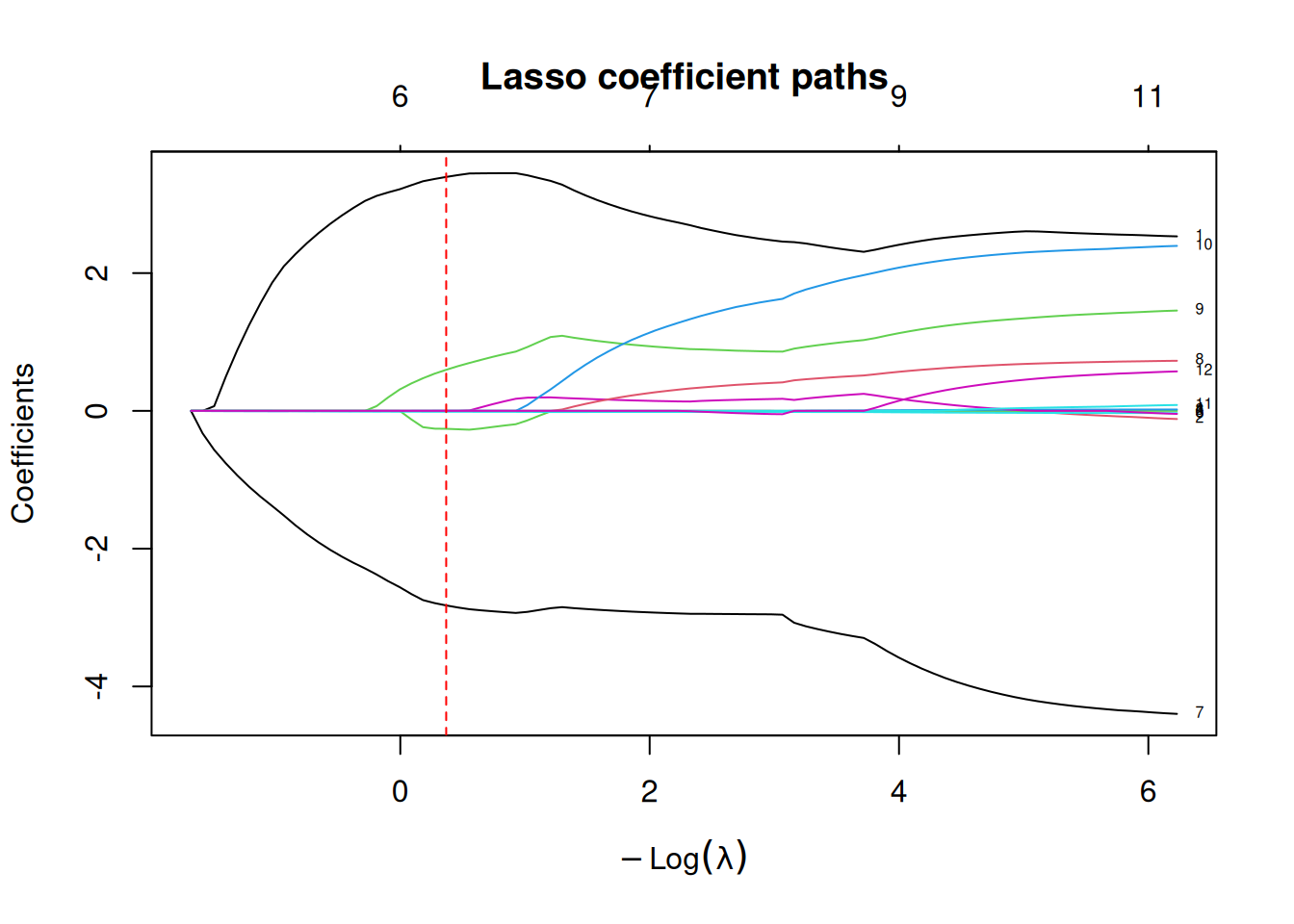

fit_ridge_path <- glmnet(X_train, y_train, alpha = 0, standardize = TRUE)
plot(fit_ridge_path, xvar = "lambda", label = FALSE, main = "Ridge coefficient paths")
abline(v = -log(cv_ridge$lambda.min), lty = 2, col = "red")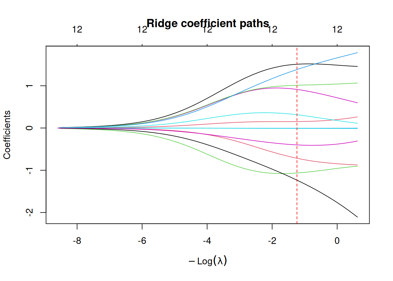

Optional: Elastic Net (alpha between 0 and 1)

If predictors are highly correlated, elastic net can outperform pure lasso.

set.seed(123)
cv_enet <- cv.glmnet(
  x = X_train,
  y = y_train,
  alpha = 0.5,          # elastic net
  nfolds = 10,
  standardize = TRUE
)

plot(cv_enet)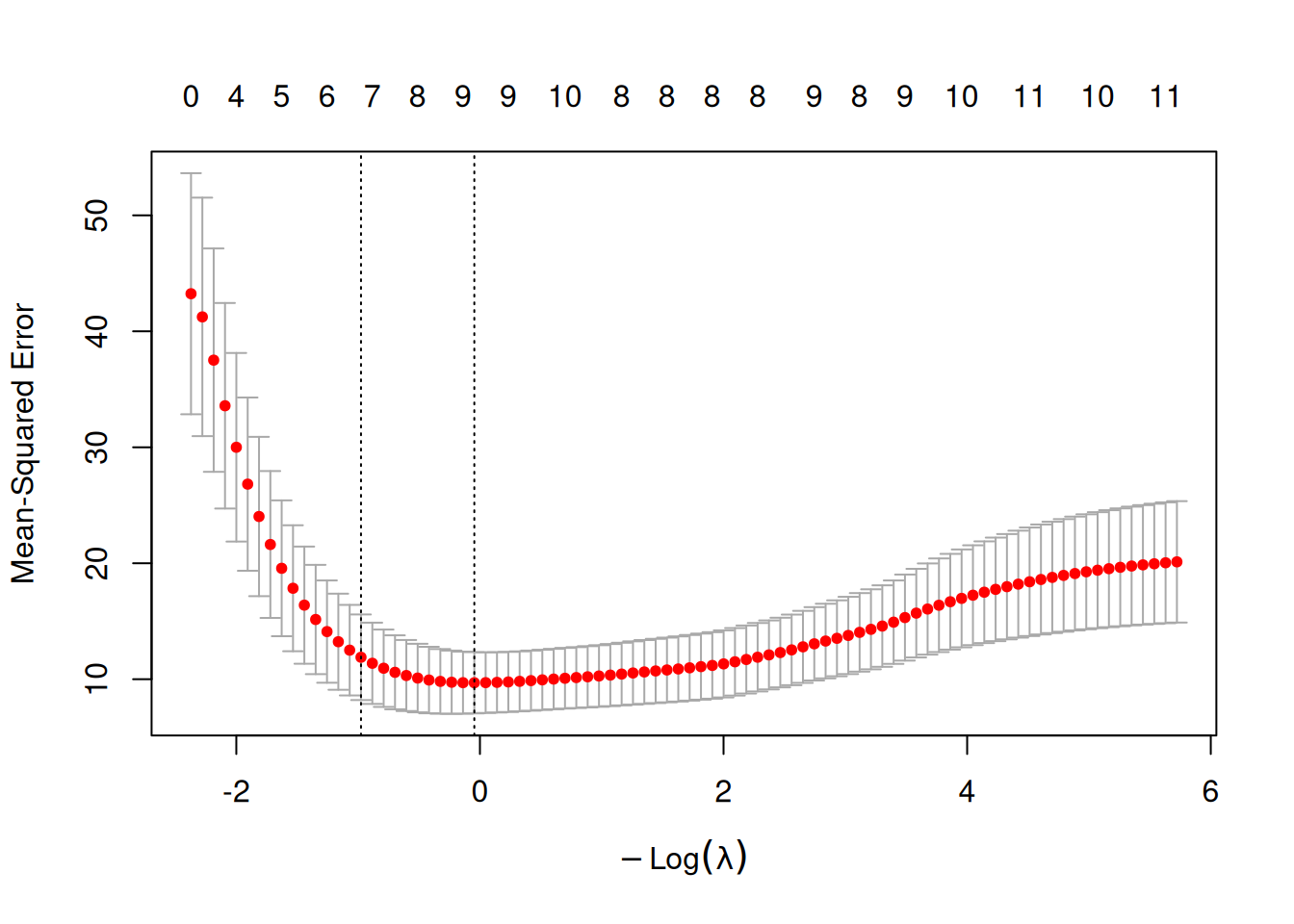

pred_enet <- predict(cv_enet, newx = X_test, s = "lambda.min")
rmse_enet <- rmse(y_test, pred_enet)

c(rmse_lasso_min = rmse_lasso_min, rmse_ridge_min = rmse_ridge_min, rmse_enet_min = rmse_enet)

## rmse_lasso_min rmse_ridge_min  rmse_enet_min 
##       2.060473       2.055639       2.077020

Best practices & warnings

Always use cross-validation for \(\lambda\); prefer lambda.min when you want stability and parsimony.
Standardization is important so that the penalty treats predictors comparably.
Lasso can be unstable when predictors are strongly correlated (it may pick one arbitrarily); elastic net is often safer.
If the goal is inference (p-values, CI), penalized regression needs extra care (post-selection inference); treat as predictive by default.

Summary

You learned how to: - Define ridge/lasso/elastic net with penalized objectives. - Fit ridge and lasso in R using glmnet + cv.glmnet(). - Select \(\lambda\) via CV (lambda.min vs lambda.1se). - Compare test RMSE and interpret shrinkage vs sparsity.

Penalized regression is a modern alternative to stepwise selection for regression problems with many correlated predictors.

A work by Gianluca Sottile

gianluca.sottile@unipa.it

Ridge & Lasso Regression in R — Penalized Linear Models with glmnet