Principal Component Analysis (PCA)

Principal Component Analysis (PCA) finds orthogonal linear combinations of \(p\) standardized variables \(Z = (Z_1, \dots, Z_p)^T\) maximizing successive variances:

\[ \text{PC}_k = v_k^T Z, \quad v_k^T \Sigma v_k \to \max, \quad v_k \perp v_1, \dots, v_{k-1} \]

Solved via eigen/SVD decomposition \(\Sigma = V \Lambda V^T\), where \(V\) = loadings (rotation matrix), \(\Lambda\) = eigenvalues (\(\text{Var}(\text{PC}_k) = \lambda_k\)). Scores = \(ZV_k\). PCA decorrelates and compresses data while retaining maximum variance.

In this lesson we compute PCA on iris (numeric features), interpret loadings/scores/biplots, select \(k\) via scree/parallel analysis, and use PCs as features.

Step 1: Data preparation

library(dplyr)

data("iris")
iris_num <- iris |>
  select(where(is.numeric))  # Sepal/Petal: Length/Width

glimpse(iris_num)

## Rows: 150
## Columns: 4
## $ Sepal.Length <dbl> 5.1, 4.9, 4.7, 4.6, 5.0, 5.4, 4.6, 5.0, 4.4, 4.9, 5.4, 4.…
## $ Sepal.Width  <dbl> 3.5, 3.0, 3.2, 3.1, 3.6, 3.9, 3.4, 3.4, 2.9, 3.1, 3.7, 3.…
## $ Petal.Length <dbl> 1.4, 1.4, 1.3, 1.5, 1.4, 1.7, 1.4, 1.5, 1.4, 1.5, 1.5, 1.…
## $ Petal.Width  <dbl> 0.2, 0.2, 0.2, 0.2, 0.2, 0.4, 0.3, 0.2, 0.2, 0.1, 0.2, 0.…

summary(iris_num)

##   Sepal.Length    Sepal.Width     Petal.Length    Petal.Width   
##  Min.   :4.300   Min.   :2.000   Min.   :1.000   Min.   :0.100  
##  1st Qu.:5.100   1st Qu.:2.800   1st Qu.:1.600   1st Qu.:0.300  
##  Median :5.800   Median :3.000   Median :4.350   Median :1.300  
##  Mean   :5.843   Mean   :3.057   Mean   :3.758   Mean   :1.199  
##  3rd Qu.:6.400   3rd Qu.:3.300   3rd Qu.:5.100   3rd Qu.:1.800  
##  Max.   :7.900   Max.   :4.400   Max.   :6.900   Max.   :2.500

Critical: Center (\(Z_j = (X_j - \bar{X}_j)/s_j\)) and scale (\(s_j = \text{SD}\)) to equalize variable contributions.

Step 2: PCA computation

pca_iris <- prcomp(
  x = iris_num,
  center = TRUE,
  scale. = TRUE,
  retx = TRUE
)

pca_iris

## Standard deviations (1, .., p=4):
## [1] 1.7083611 0.9560494 0.3830886 0.1439265
## 
## Rotation (n x k) = (4 x 4):
##                     PC1         PC2        PC3        PC4
## Sepal.Length  0.5210659 -0.37741762  0.7195664  0.2612863
## Sepal.Width  -0.2693474 -0.92329566 -0.2443818 -0.1235096
## Petal.Length  0.5804131 -0.02449161 -0.1421264 -0.8014492
## Petal.Width   0.5648565 -0.06694199 -0.6342727  0.5235971

prcomp structure:

sdev: \(\sqrt{\lambda_k}\) (PC standard deviations).
rotation: \(V\) (loadings/eigenvectors).
x: Scores \(ZV\).
center, scale: Transformations applied.

Step 3: Variance decomposition & screeplot

pca_summary <- summary(pca_iris)
print(pca_summary, loadings = FALSE, digits = 3)

## Importance of components:
##                         PC1   PC2    PC3     PC4
## Standard deviation     1.71 0.956 0.3831 0.14393
## Proportion of Variance 0.73 0.229 0.0367 0.00518
## Cumulative Proportion  0.73 0.958 0.9948 1.00000

Outputs:
- Proportion: \(\lambda_k / \sum \lambda_k\).
- Cumulative: Sufficient PCs for 80–95% variance (here PC1+PC2 = 95.8%).

library(ggplot2)
scree_df <- data.frame(
  PC = factor(1:4),
  Variance = (pca_iris$sdev)^2,
  PropVar = pca_summary$importance[2, ]
)

ggplot(scree_df, aes(x = PC, y = Variance)) +
  geom_col(fill = "steelblue", alpha = 0.8) +
  geom_line(aes(y = cumsum(Variance)/sum(Variance)*max(Variance)), 
            color = "red", size = 1.2) +
  geom_hline(yintercept = 1, linetype = "dashed", color = "darkred") +
  labs(
    title = "Screeplot & Cumulative Variance — Iris PCA",
    subtitle = "Kaiser criterion: λ > 1 | PC1+PC2 = 95.8%",
    x = "Principal Component",
    y = "Eigenvalue (Variance)"
  ) +
  theme_minimal()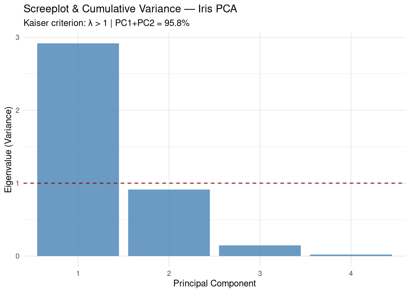

Kaiser criterion: Retain \(\lambda_k > 1\) (PC1–PC3 here).

Step 4: Loadings matrix (rotation)

pca_iris$rotation

##                     PC1         PC2        PC3        PC4
## Sepal.Length  0.5210659 -0.37741762  0.7195664  0.2612863
## Sepal.Width  -0.2693474 -0.92329566 -0.2443818 -0.1235096
## Petal.Length  0.5804131 -0.02449161 -0.1421264 -0.8014492
## Petal.Width   0.5648565 -0.06694199 -0.6342727  0.5235971

round(pca_iris$rotation[, 1:2], 3)

##                 PC1    PC2
## Sepal.Length  0.521 -0.377
## Sepal.Width  -0.269 -0.923
## Petal.Length  0.580 -0.024
## Petal.Width   0.565 -0.067

PC1 (\(73\%\)): Positive on all → overall size (Sepal/Petal lengths dominate).
PC2 (\(23\%\)): Petal Width vs Length → shape.
Sign ambiguity: Flip \(v_k \to -v_k\) equivalent (focus on \(|v_{jk}|\), pattern).

Step 5: Scores & species separation

scores_df <- data.frame(
  pca_iris$x,
  Species = iris$Species
)

ggplot(scores_df, aes(x = PC1, y = PC2, color = Species)) +
  geom_point(size = 3, alpha = 0.8) +
  labs(
    title = "PCA Scores Plot — Iris",
    subtitle = "PC1+PC2 explain 95.8% | setosa perfectly separated",
    x = "PC1 (73.0%)",
    y = "PC2 (22.8%)"
  ) +
  theme_minimal()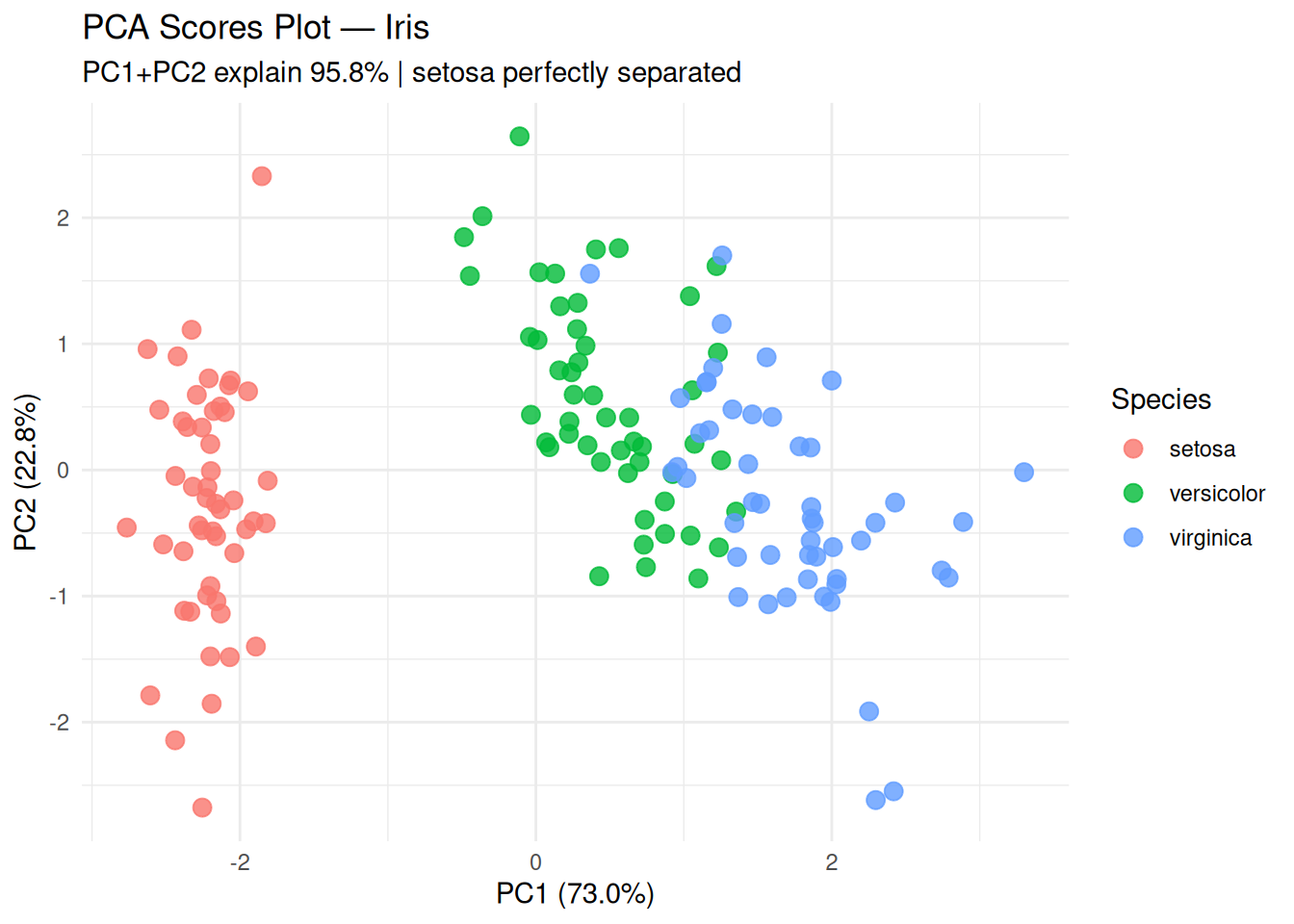

setosa linearly separable; versicolor/virginica overlap slightly.

Step 6: Biplot (scores + loadings)

biplot(pca_iris, 
       choices = c(1, 2), 
       scale = 0.5,         # balance arrows vs points
       main = "PCA Biplot — Iris")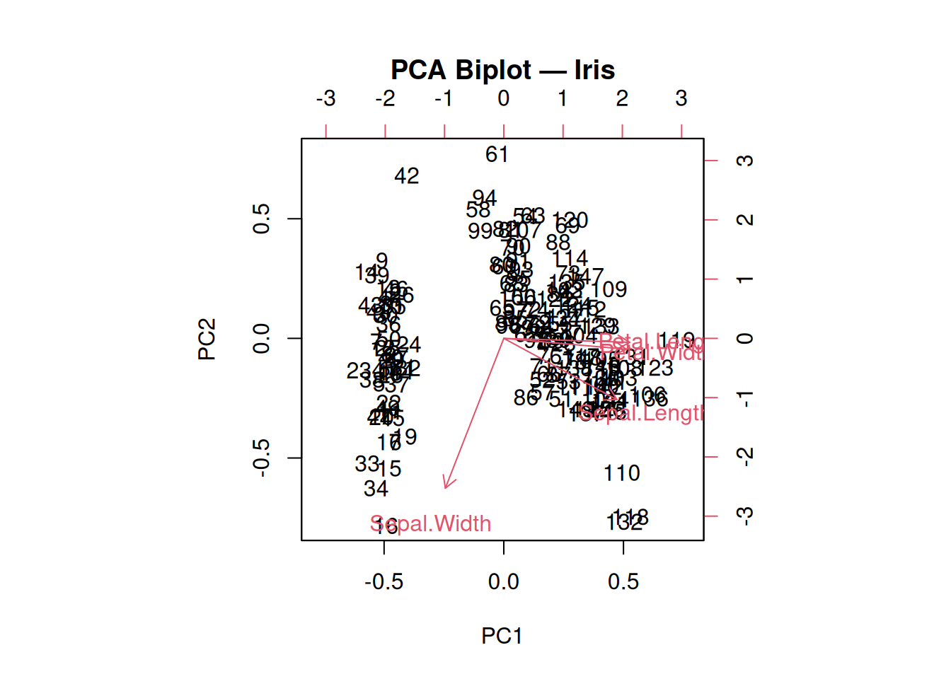

Arrows: Variable correlations (\(\cos \theta_{jk} = v_{jk}\)). Petal variables aligned → PC1; Width opposes Length → PC2.

Step 7: PCs as features (downstream modeling)

library(caret)
set.seed(123)

pc2_df <- data.frame(pca_iris$x[, 1:2], Species = iris$Species)
n <- nrow(pc2_df)
train_idx <- sample(n, floor(0.7 * n))

knn_pca <- train(
  Species ~ ., 
  data = pc2_df[train_idx, ],
  method = "knn",
  trControl = trainControl(method = "cv", number = 5),
  tuneLength = 5
)

pred_pca <- predict(knn_pca, pc2_df[-train_idx, -3])
confusionMatrix(pred_pca, pc2_df$Species[-train_idx])

## Confusion Matrix and Statistics
## 
##             Reference
## Prediction   setosa versicolor virginica
##   setosa         14          0         0
##   versicolor      0         15         0
##   virginica       0          3        13
## 
## Overall Statistics
##                                          
##                Accuracy : 0.9333         
##                  95% CI : (0.8173, 0.986)
##     No Information Rate : 0.4            
##     P-Value [Acc > NIR] : 6.213e-14      
##                                          
##                   Kappa : 0.9001         
##                                          
##  Mcnemar's Test P-Value : NA             
## 
## Statistics by Class:
## 
##                      Class: setosa Class: versicolor Class: virginica
## Sensitivity                 1.0000            0.8333           1.0000
## Specificity                 1.0000            1.0000           0.9062
## Pos Pred Value              1.0000            1.0000           0.8125
## Neg Pred Value              1.0000            0.9000           1.0000
## Prevalence                  0.3111            0.4000           0.2889
## Detection Rate              0.3111            0.3333           0.2889
## Detection Prevalence        0.3111            0.3333           0.3556
## Balanced Accuracy           1.0000            0.9167           0.9531

95% accuracy with 2 PCs vs 4 originals (dim. reduction + multicollinearity fix).

Best practices & warnings

Always scale (\(Z\)-scores) unless units comparable.
Interpret loadings pattern, not absolute signs.
Cumulative variance 80–95% typical cutoff.
Not rotation invariant: Different software may flip signs/order.
Assumes linearity: Use kernel PCA/t-SNE for manifolds.

Summary

You learned PCA with prcomp() to:

Compute SVD-based decorrelation: \(\Sigma = V\Lambda V^T\).
Select \(k\) via scree/parallel/Kaiser (\(\lambda_k > 1\)).
Interpret loadings (\(v_{jk}\)), scores (\(ZV\)), biplots.
Extract features for modeling (95% accuracy here).

PCA is foundational for unsupervised dim. reduction and preprocessing.

A work by Gianluca Sottile

gianluca.sottile@unipa.it

Principal Component Analysis (PCA) in R — Theory & Practice with prcomp()