Factor Analysis (FA) in R — Latent Factors with psych::fa()
Factor Analysis (FA)
Factor Analysis posits a measurement model where \(p\) observed variables \(X = (X_1, \dots, X_p)^T\) are linear combinations of \(m < p\) latent factors \(F = (F_1, \dots, F_m)^T\) plus unique errors \(\epsilon\):
\[ X = \Lambda F + \epsilon, \quad \text{Cov}(\epsilon) = \Psi \text{(diagonal)} \]
\(\Lambda\) contains factor loadings, \(\Psi_{ii}\) unique variances. FA estimates common variance (communalities \(h^2_i = 1 - \psi_{ii}\)), maximizing likelihood under normality assumptions. Unlike PCA (total variance), FA focuses on shared covariance structure (psychometrics, questionnaire validation).
In this lesson we fit the Big Five model to
bfi (25 personality items), validate factorability,
interpret rotated loadings, and assess fit.
Step 1: Data preparation and factorability tests
library(psych)
library(dplyr)

data("bfi")
bfi_num <- bfi |>
  select(A1:A5, C1:C5, E1:E5, N1:N5, O1:O5) |>  # 5 scales × 5 items
  na.omit()

glimpse(bfi_num)
## Rows: 2,436
## Columns: 25
## $ A1 <int> 2, 2, 5, 4, 2, 6, 2, 4, 2, 4, 5, 5, 4, 4, 4, 5, 4, 4, 5, 1, 1, 2, 4…
## $ A2 <int> 4, 4, 4, 4, 3, 6, 5, 3, 5, 4, 5, 5, 5, 3, 6, 5, 4, 4, 4, 6, 5, 6, 5…
## $ A3 <int> 3, 5, 5, 6, 3, 5, 5, 1, 6, 5, 5, 5, 2, 6, 6, 5, 5, 6, 2, 6, 6, 5, 5…
## $ A4 <int> 4, 2, 4, 5, 4, 6, 3, 5, 6, 6, 6, 6, 2, 6, 2, 4, 4, 5, 1, 1, 5, 6, 6…
## $ A5 <int> 4, 5, 4, 5, 5, 5, 5, 1, 5, 5, 4, 6, 1, 3, 5, 5, 3, 5, 2, 5, 6, 5, 5…
## $ C1 <int> 2, 5, 4, 4, 4, 6, 5, 3, 6, 4, 5, 4, 5, 5, 4, 5, 5, 1, 4, 5, 4, 3, 5…
## $ C2 <int> 3, 4, 5, 4, 4, 6, 4, 2, 5, 3, 4, 4, 5, 5, 4, 5, 4, 1, 6, 4, 3, 5, 5…
## $ C3 <int> 3, 4, 4, 3, 5, 6, 4, 4, 6, 5, 3, 4, 5, 5, 4, 5, 5, 1, 5, 4, 2, 6, 4…
## $ C4 <int> 4, 3, 2, 5, 3, 1, 2, 2, 2, 3, 2, 2, 2, 3, 4, 4, 4, 5, 5, 2, 4, 3, 1…
## $ C5 <int> 4, 4, 5, 5, 2, 3, 3, 4, 1, 2, 2, 1, 2, 5, 4, 3, 6, 6, 4, 3, 5, 6, 1…
## $ E1 <int> 3, 1, 2, 5, 2, 2, 4, 3, 2, 1, 3, 2, 3, 1, 1, 2, 1, 1, 3, 1, 2, 2, 3…
## $ E2 <int> 3, 1, 4, 3, 2, 1, 3, 6, 2, 3, 3, 2, 4, 1, 2, 2, 2, 1, 3, 2, 1, 2, 2…
## $ E3 <int> 3, 6, 4, 4, 5, 6, 4, 4, 4, 2, 3, 4, 3, 6, 5, 4, 4, 4, 5, 4, 2, 4, 5…
## $ E4 <int> 4, 4, 4, 4, 4, 5, 5, 2, 5, 5, 2, 6, 6, 6, 5, 6, 5, 5, 5, 3, 5, 6, 5…
## $ E5 <int> 4, 3, 5, 4, 5, 6, 5, 1, 5, 4, 4, 5, 5, 4, 5, 6, 5, 6, 4, 4, 2, 6, 6…
## $ N1 <int> 3, 3, 4, 2, 2, 3, 1, 6, 5, 3, 1, 1, 2, 4, 4, 6, 5, 5, 1, 2, 2, 4, 2…
## $ N2 <int> 4, 3, 5, 5, 3, 5, 2, 3, 5, 3, 2, 1, 4, 5, 4, 5, 6, 5, 3, 5, 2, 4, 3…
## $ N3 <int> 2, 3, 4, 2, 4, 2, 2, 2, 5, 4, 2, 1, 2, 4, 4, 5, 5, 5, 3, 5, 2, 4, 3…
## $ N4 <int> 2, 5, 2, 4, 4, 2, 1, 6, 2, 2, 2, 2, 2, 5, 4, 4, 5, 1, 2, 4, 2, 6, 1…
## $ N5 <int> 3, 5, 3, 1, 3, 3, 1, 4, 4, 3, 2, 1, 3, 5, 5, 4, 2, 1, 1, 6, 2, 6, 1…
## $ O1 <int> 3, 4, 4, 3, 3, 4, 5, 3, 5, 5, 4, 5, 5, 6, 5, 5, 4, 4, 6, 5, 6, 6, 6…
## $ O2 <int> 6, 2, 2, 3, 3, 3, 2, 2, 1, 3, 2, 3, 2, 6, 1, 1, 2, 1, 1, 1, 1, 1, 2…
## $ O3 <int> 3, 4, 5, 4, 4, 5, 5, 4, 5, 5, 4, 4, 5, 6, 5, 4, 2, 5, 3, 6, 5, 5, 5…
## $ O4 <int> 4, 3, 5, 3, 3, 6, 6, 5, 5, 6, 5, 4, 5, 3, 6, 5, 4, 3, 2, 6, 5, 6, 6…
## $ O5 <int> 3, 3, 2, 5, 3, 1, 1, 3, 2, 3, 2, 4, 5, 2, 3, 4, 2, 2, 4, 2, 2, 1, 2…## A1 A2 A3 A4 A5 C1
## A1 1.00 -0.35 -0.27 -0.16 -0.19 0.01
## A2 -0.35 1.00 0.50 0.35 0.40 0.10
## A3 -0.27 0.50 1.00 0.38 0.52 0.11
## A4 -0.16 0.35 0.38 1.00 0.33 0.09
## A5 -0.19 0.40 0.52 0.33 1.00 0.13
## C1 0.01 0.10 0.11 0.09 0.13 1.00Step 2: Factorability assessment (KMO + Bartlett)
## Kaiser-Meyer-Olkin factor adequacy
## Call: KMO(r = bfi_num)
## Overall MSA =  0.85
## MSA for each item =
##   A1   A2   A3   A4   A5   C1   C2   C3   C4   C5   E1   E2   E3   E4   E5   N1
## 0.75 0.84 0.87 0.88 0.90 0.84 0.80 0.85 0.83 0.86 0.84 0.88 0.90 0.88 0.89 0.78
##   N2   N3   N4   N5   O1   O2   O3   O4   O5
## 0.78 0.86 0.89 0.86 0.86 0.78 0.84 0.77 0.76## $chisq
## [1] 18146.07
##
## $p.value
## [1] 0
##
## $df
## [1] 300KMO = 0.85, Bartlett \(p < 2.2e-16\): Excellent factorability (significant correlations, adequate sample communalities).
Step 3: Fit 5-factor model (ML estimation)
fa_bfi <- fa(
  r = bfi_num,              # raw data (correlations auto-computed)
  nfactors = 5,             # Big Five theory
  rotate = "varimax",       # orthogonal rotation (simple structure)
  fm = "ml",                # maximum likelihood
  max.iter = 1000
)

print(fa_bfi)
## Factor Analysis using method = ml
## Call: fa(r = bfi_num, nfactors = 5, rotate = "varimax", max.iter = 1000,
## fm = "ml")
## Standardized loadings (pattern matrix) based upon correlation matrix
## ML2 ML1 ML3 ML5 ML4 h2 u2 com
## A1 0.10 0.05 0.00 -0.39 -0.06 0.17 0.83 1.2
## A2 0.04 0.19 0.14 0.60 0.06 0.42 0.58 1.4
## A3 0.02 0.28 0.11 0.66 0.06 0.53 0.47 1.4
## A4 -0.06 0.18 0.23 0.45 -0.11 0.31 0.69 2.0
## A5 -0.12 0.35 0.08 0.58 0.08 0.49 0.51 1.8
## C1 0.00 0.05 0.53 0.06 0.22 0.34 0.66 1.4
## C2 0.08 0.01 0.62 0.13 0.14 0.43 0.57 1.2
## C3 -0.03 0.01 0.55 0.12 0.00 0.32 0.68 1.1
## C4 0.22 -0.08 -0.65 -0.02 -0.09 0.49 0.51 1.3
## C5 0.27 -0.19 -0.57 -0.05 0.04 0.44 0.56 1.7
## E1 0.03 -0.59 0.03 -0.12 -0.07 0.37 0.63 1.1
## E2 0.23 -0.67 -0.11 -0.15 -0.06 0.55 0.45 1.4
## E3 0.02 0.49 0.07 0.31 0.31 0.44 0.56 2.5
## E4 -0.12 0.61 0.09 0.36 -0.04 0.53 0.47 1.8
## E5 0.05 0.49 0.31 0.12 0.23 0.41 0.59 2.4
## N1 0.82 0.09 -0.04 -0.21 -0.08 0.73 0.27 1.2
## N2 0.79 0.04 -0.02 -0.20 -0.02 0.66 0.34 1.1
## N3 0.71 -0.08 -0.08 -0.02 0.00 0.52 0.48 1.1
## N4 0.56 -0.37 -0.19 0.00 0.07 0.49 0.51 2.0
## N5 0.52 -0.19 -0.05 0.11 -0.14 0.34 0.66 1.5
## O1 -0.01 0.18 0.10 0.09 0.52 0.33 0.67 1.4
## O2 0.16 0.00 -0.11 0.10 -0.45 0.26 0.74 1.5
## O3 0.02 0.28 0.07 0.15 0.61 0.48 0.52 1.6
## O4 0.21 -0.22 -0.03 0.14 0.37 0.25 0.75 2.7
## O5 0.08 -0.01 -0.08 0.01 -0.51 0.27 0.73 1.1
##
## ML2 ML1 ML3 ML5 ML4
## SS loadings 2.69 2.32 2.03 1.98 1.56
## Proportion Var 0.11 0.09 0.08 0.08 0.06
## Cumulative Var 0.11 0.20 0.28 0.36 0.42
## Proportion Explained 0.25 0.22 0.19 0.19 0.15
## Cumulative Proportion 0.25 0.47 0.67 0.85 1.00
##
## Mean item complexity = 1.6
## Test of the hypothesis that 5 factors are sufficient.
##
## df null model = 300 with the objective function = 7.48 with Chi Square = 18146.07
## df of the model are 185 and the objective function was 0.62
##
## The root mean square of the residuals (RMSR) is 0.03
## The df corrected root mean square of the residuals is 0.04
##
## The harmonic n.obs is 2436 with the empirical chi square 598.49 with prob < 4.4e-45
## The total n.obs was 2436 with Likelihood Chi Square = 1490.59 with prob < 1.2e-202
##
## Tucker Lewis Index of factoring reliability = 0.881
## RMSEA index = 0.054 and the 90 % confidence intervals are 0.051 0.056
## BIC = 47.94
## Fit based upon off diagonal values = 0.98
## Measures of factor score adequacy
## ML2 ML1 ML3 ML5 ML4
## Correlation of (regression) scores with factors 0.93 0.87 0.86 0.85 0.83
## Multiple R square of scores with factors 0.86 0.76 0.74 0.72 0.69
## Minimum correlation of possible factor scores 0.73 0.51 0.49 0.45 0.37Fit indices: - TLI > 0.88:
Excellent incremental fit.
- RMSEA < 0.06: Good absolute fit.
Step 4: Screeplot (parallel analysis)
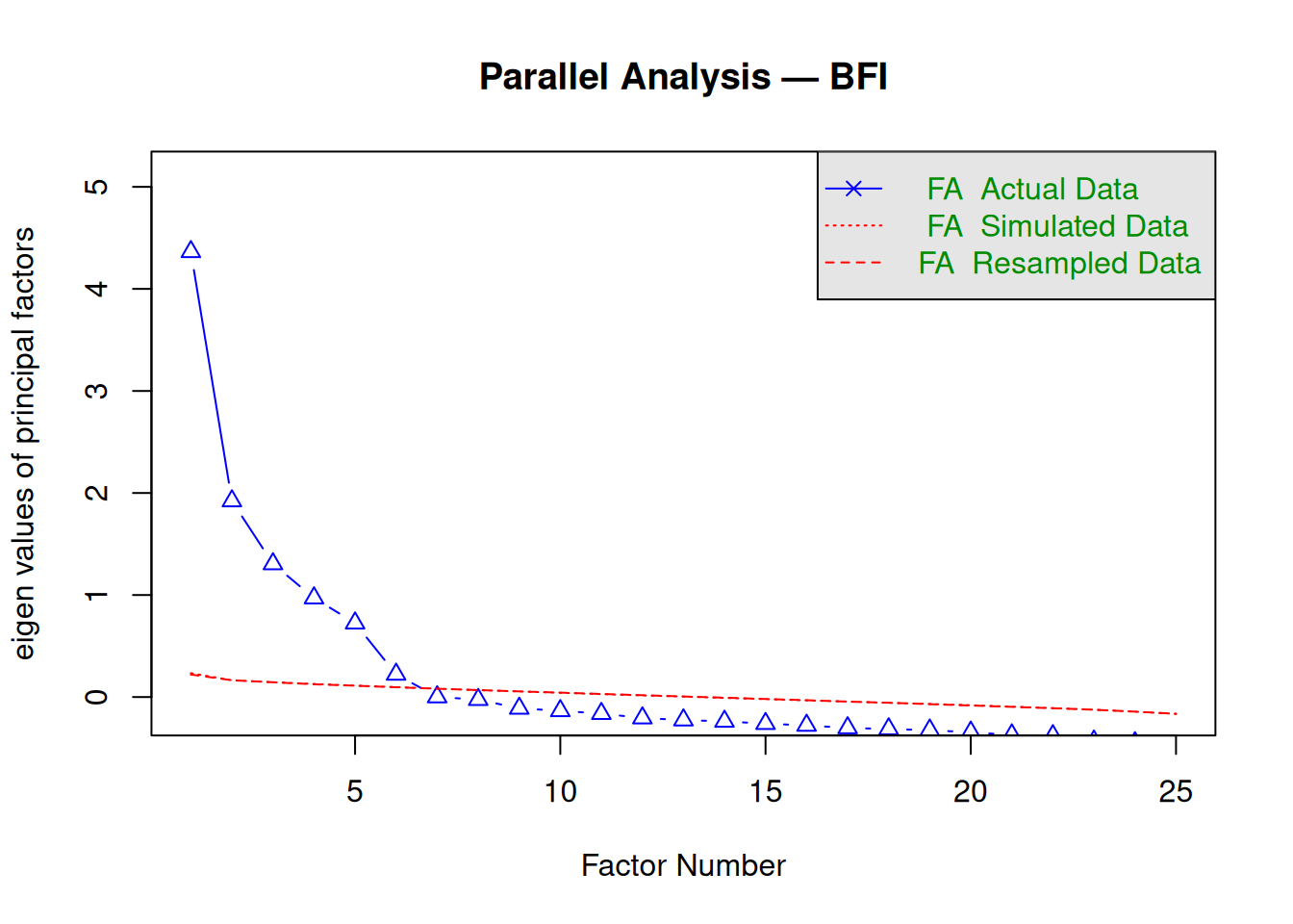
## Parallel analysis suggests that the number of factors = 6 and the number of components = NAParallel analysis suggests 6 factors (eigenvalues exceed random data).
Step 5: Rotated loadings (pattern matrix)
##
## Loadings:
##    ML2    ML1    ML3    ML5    ML4
## A1
## A2                       0.601
## A3                       0.662
## A4                       0.454
## A5                       0.580
## C1                0.533
## C2                0.624
## C3                0.554
## C4               -0.653
## C5               -0.573
## E1        -0.587
## E2        -0.674
## E3         0.490
## E4         0.613
## E5         0.491
## N1  0.816
## N2  0.787
## N3  0.714
## N4  0.562
## N5  0.518
## O1                              0.524
## O2                             -0.454
## O3                              0.614
## O4
## O5                             -0.512
##
##                  ML2   ML1   ML3   ML5   ML4
## SS loadings    2.687 2.320 2.034 1.978 1.557
## Proportion Var 0.107 0.093 0.081 0.079 0.062
## Cumulative Var 0.107 0.200 0.282 0.361 0.423
Interpretation (varimax rotation):
- MR1: High on A1–A5 →
Agreeableness.
- MR2: C1–C5 →
Conscientiousness.
- Loadings \(|> 0.4|\) define salient items; cross-loadings minimal (good simple structure).
Communalities \(h^2\):
##    A1    A2    A3    A4    A5    C1    C2    C3    C4    C5    E1    E2    E3
## 0.170 0.424 0.534 0.309 0.488 0.340 0.431 0.323 0.490 0.443 0.366 0.546 0.442
##    E4    E5    N1    N2    N3    N4    N5    O1    O2    O3    O4    O5
## 0.532 0.408 0.729 0.663 0.522 0.493 0.336 0.325 0.256 0.482 0.248 0.274
Mean \(h^2 = 0.42\): Moderate common variance (adequate for personality scales).
Step 6: Factor diagram and uniqueness
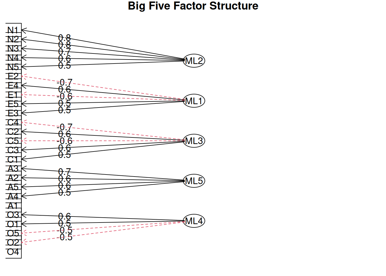
Uniqueness \(\psi_{ii} = 1 - h_i^2\): High values indicate item specificity.
Step 7: Model comparison — PCA vs FA loadings
pca_bfi <- principal(bfi_num, nfactors = 5, rotate = "varimax")
print(pca_bfi$loadings, cutoff = 0.4)
##
## Loadings:
## RC2 RC1 RC3 RC5 RC4
## A1 -0.638
## A2 0.716
## A3 0.688
## A4 0.530
## A5 0.436 0.572
## C1 0.654
## C2 0.738
## C3 0.679
## C4 -0.692
## C5 -0.627
## E1 -0.680
## E2 -0.722
## E3 0.626
## E4 0.700
## E5 0.586
## N1 0.806
## N2 0.794
## N3 0.794
## N4 0.649
## N5 0.631
## O1 0.598
## O2 -0.606
## O3 0.640
## O4 0.494
## O5 -0.677
##
## RC2 RC1 RC3 RC5 RC4
## SS loadings 3.185 3.103 2.619 2.375 2.148
## Proportion Var 0.127 0.124 0.105 0.095 0.086
## Cumulative Var 0.127 0.251 0.356 0.451 0.537## FA RMSR: 0.029## PCA RMSR: 0.04FA RMSR < PCA: Better reproduction of correlations (focus on covariance vs total variance).
Summary
You learned FA with psych::fa() to:
- Model \(X = \Lambda F + \epsilon\)
via maximum likelihood.
- Validate with KMO/Bartlett, parallel analysis,
TLI/RMSEA.
- Interpret varimax loadings, \(h^2\), and compare to PCA.
FA uncovers latent constructs when theory suggests unobserved common causes.
A work by Gianluca Sottile
gianluca.sottile@unipa.it