Spectral Clustering

Spectral clustering is a graph-based method. It builds an affinity graph \(W\) from similarities (e.g., RBF kernel): \(W_{ij} = \exp(-\|x_i - x_j\|^2 / (2\sigma^2))\).

Define the degree matrix \(D\) where \(D_{ii} = \sum_j W_{ij}\), and (one version of) the normalized Laplacian: \(L = I - D^{-1/2} W D^{-1/2}\).

The algorithm embeds data into the space spanned by a few eigenvectors of \(L\) (or a related matrix) and then runs a simple clustering method (often K-means) in that embedding.

This family is particularly useful when clusters are not well-separated in Euclidean space but are separable by connectivity on a similarity graph.

In this lesson:

Fit spectral clustering with an RBF kernel.
Tune the kernel scale \(\sigma\) pragmatically.
Compare with K-means/hierarchical results.

Step 1: Import + preprocessing

library(readr)
library(dplyr)

local_path <- "raw_data/wholesale_customers.csv"
df_raw <- read_csv(local_path, show_col_types = FALSE)

spend_vars <- c("Fresh", "Milk", "Grocery", "Frozen", "Detergents_Paper", "Delicassen")

X <- df_raw |>
  mutate(across(all_of(spend_vars), ~ log1p(.x))) |>
  select(all_of(spend_vars)) |>
  mutate(across(everything(), scale)) |>
  as.matrix()

Step 2: Choose k (reuse from prior analyses or evaluate a grid)

Spectral clustering typically requires specifying \(k\). Here we illustrate a simple approach: test a small grid and select based on silhouette in the embedded labels.

library(cluster)
library(kernlab)

avg_sil_from_labels <- function(X, labels) {
  if (length(unique(labels)) < 2) return(NA_real_)
  s <- silhouette(labels, dist(X))
  mean(s[, 3])
}

k_grid <- 2:10
sigma_grid <- c(0.1, 0.2, 0.5, 1)

results <- expand.grid(k = k_grid, sigma = sigma_grid)
results$avg_sil <- NA_real_

set.seed(123)
for (i in seq_len(nrow(results))) {
  k <- results$k[i]
  sig <- results$sigma[i]
  
  sc <- specc(X, centers = k, kernel = "rbfdot", kpar = list(sigma = sig))
  results$avg_sil[i] <- avg_sil_from_labels(X, as.integer(sc))
}

results <- results[order(-results$avg_sil), ]
head(results, 10)

	k	sigma	avg_sil
28	2	1.0	0.2897449
10	2	0.2	0.2892797
19	2	0.5	0.2888352
1	2	0.1	0.2868777
11	3	0.2	0.2498515
2	3	0.1	0.2071218
12	4	0.2	0.1920744
21	4	0.5	0.1790377
3	4	0.1	0.1777185
5	6	0.1	0.1729661

Select the best configuration (highest silhouette), and then refit:

best_k <- results$k[1]
best_sigma <- results$sigma[1]

set.seed(123)
sc_best <- specc(X, centers = best_k, kernel = "rbfdot", kpar = list(sigma = best_sigma))
cl_sc <- as.integer(sc_best)

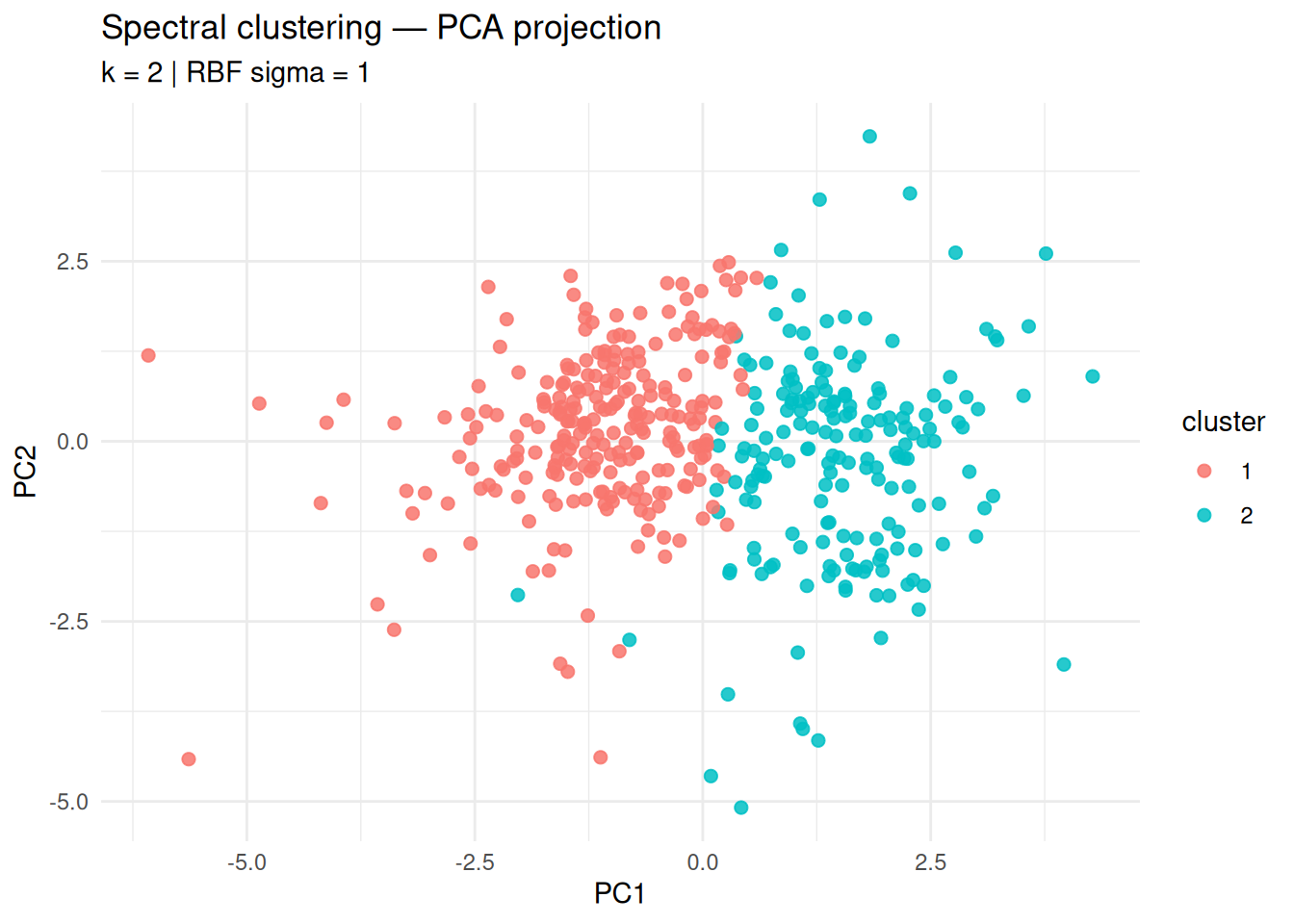
table(cl_sc)

## cl_sc
##   1   2 
## 254 186

Step 3: Visualization (PCA projection)

library(ggplot2)

pc <- prcomp(X)
plot_df <- data.frame(
  PC1 = pc$x[, 1],
  PC2 = pc$x[, 2],
  cluster = factor(cl_sc)
)

ggplot(plot_df, aes(PC1, PC2, color = cluster)) +
  geom_point(size = 2, alpha = 0.85) +
  theme_minimal() +
  labs(
    title = "Spectral clustering — PCA projection",
    subtitle = paste("k =", best_k, "| RBF sigma =", best_sigma),
    x = "PC1", y = "PC2"
  )

Step 4: Comparison with K-means (same k)

library(mclust)

set.seed(123)
km <- kmeans(X, centers = best_k, nstart = 50)

ari <- adjustedRandIndex(cl_sc, km$cluster)
ari

## [1] 0.893599

Interpretation:

Spectral clustering is preferred when K-means struggles due to non-convex or graph-structured clusters.
If ARI is high, it suggests the structure is already well captured by centroid-based clustering.

Step 5: Cluster profiles

df_prof <- as.data.frame(X)
df_prof$cluster <- factor(cl_sc)

profiles <- df_prof |>
  group_by(cluster) |>
  summarize(across(where(is.numeric), mean), .groups = "drop")

profiles

cluster	Fresh	Milk	Grocery	Frozen	Detergents_Paper	Delicassen
1	0.2152193	-0.5720568	-0.6377129	0.2678828	-0.6509132	-0.1329263
2	-0.2939016	0.7811958	0.8708552	-0.3658184	0.8888815	0.1815230

Summary

Spectral clustering works on a similarity graph and can capture structures that are not well modeled by spherical clusters.
The kernel scale \(\sigma\) is crucial; a small grid search with an internal index (e.g., silhouette) is a practical approach.
Compare against K-means to justify switching clustering families rather than forcing centroid-based methods.

A work by Gianluca Sottile

gianluca.sottile@unipa.it