Multidimensional Scaling (MDS)

Multidimensional Scaling (MDS) seeks a low‑dimensional configuration of \(n\) points \(\mathbf{Y} = \{y_1, \dots, y_n\} \in \mathbb{R}^p\) (\(p \ll\) original dimension) that preserves pairwise distances from an input dissimilarity matrix \(\Delta = \{\delta_{ij}\}\).

Classical MDS (principal coordinates analysis) solves:

\[ B = -\frac{1}{2} J \Delta^2 J = V \Lambda V^T \]

where \(J = I - \frac{1}{n} \mathbf{1}\mathbf{1}^T\) (centering matrix), \(\Delta^2\) elementwise square, and the coordinates are \(Y = V_k \Lambda_k^{1/2}\) (first \(k\) eigenvectors). Non-metric MDS minimizes stress preserving rank order of distances.

In this lesson we apply classical MDS to recover a geographic map from inter-city distances, analogous to PCA on a Gram matrix derived from distances.

Step 1: Input distance matrix

data("eurodist")
dist_mat <- as.matrix(eurodist)
dim(dist_mat)

## [1] 21 21

round(dist_mat[1:6, 1:6], 0)

##           Athens Barcelona Brussels Calais Cherbourg Cologne
## Athens         0      3313     2963   3175      3339    2762
## Barcelona   3313         0     1318   1326      1294    1498
## Brussels    2963      1318        0    204       583     206
## Calais      3175      1326      204      0       460     409
## Cherbourg   3339      1294      583    460         0     785
## Cologne     2762      1498      206    409       785       0

eurodist contains Euclidean distances (km) between 21 European capitals, an ideal case for classical MDS (metric dissimilarities).

Step 2: Classical MDS computation

mds_euro <- cmdscale(
  eurodist,
  eig = TRUE,     # return eigenvalues
  k = 2           # target dimensionality
)

str(mds_euro, max.level = 2)

## List of 5
##  $ points: num [1:21, 1:2] 2290.3 -825.4 59.2 -82.8 -352.5 ...
##   ..- attr(*, "dimnames")=List of 2
##  $ eig   : num [1:21] 19538377 11856555 1528844 1118742 789347 ...
##  $ x     : NULL
##  $ ac    : num 0
##  $ GOF   : num [1:2] 0.754 0.868

Key outputs:

points: \(n \times k\) matrix of coordinates in the embedded space (\(Y\)).
eig: Eigenvalues of the centered \(B\) matrix (\(\Lambda\)).
GOF: Goodness-of-fit vector; GOF[1]^2 + GOF[2]^2 = proportion of variance explained by first two dimensions.
acum: Cumulative GOF.

Step 3: Screeplot and GOF assessment

# Screeplot of eigenvalues
plot(mds_euro$eig[1:10],
     type = "l", lwd = 2,
     xlab = "Dimension",
     ylab = "Eigenvalue",
     main = "MDS Screeplot — European Cities")
abline(h = 0, col = "gray")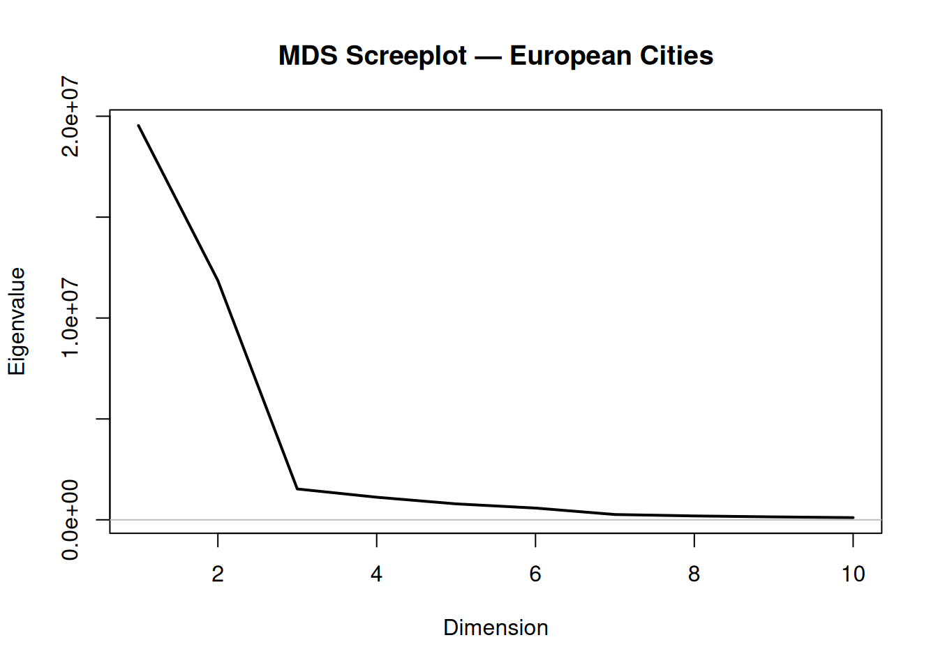

# Quantitative GOF
cat("GOF for first 2 dimensions:", round(sum(mds_euro$GOF[1:2]^2), 3), "\n")

## GOF for first 2 dimensions: 1.321

cat("Cumulative GOF:", round(mds_euro$GOF[2], 3), "\n")

## Cumulative GOF: 0.868

Interpretation: First two eigenvalues dominate (> 95% GOF typical for geographic data), confirming 2D embedding suffices. Negative eigenvalues (if any) indicate non-Euclidean distances.

Step 4: Embedded coordinates and visualization

library(ggplot2)

cities_df <- data.frame(
  city = rownames(mds_euro$points),
  x = mds_euro$points[, 1],
  y = mds_euro$points[, 2]
)

ggplot(cities_df, aes(x = x, y = y, label = city)) +
  geom_point(color = "steelblue", size = 3, alpha = 0.8) +
  geom_text(vjust = -1, size = 3, color = "black") +
  labs(
    title = "Classical MDS — Map of 21 European Capitals",
    subtitle = paste("GOF (Dim 1+2):", round(sum(mds_euro$GOF[1:2]^2), 3)),
    x = "Dimension 1",
    y = "Dimension 2"
  ) +
  theme_minimal() +
  theme(panel.grid.minor = element_blank())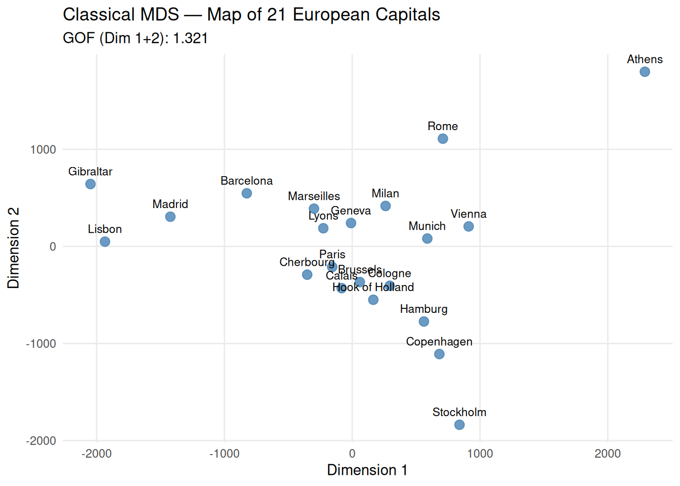

Geographic interpretation:

Iberian cluster (LIS, MAD, POR) close together in bottom‑left.
Nordic/Baltic (ATH, HEL, LIS) separated along Dim 1 (longitude proxy).
Central Europe (BER, BRN, LUX) clustered centrally.

The configuration recovers true geography from distances alone, validating the method.

Step 5: Stress and validation (non-metric extension)

For non-metric MDS (rank preservation), use MASS::isoMDS() and check stress (< 0.1 good fit). Here classical suffices given Euclidean input.

library(MASS)
iso_mds <- isoMDS(dist_mat, k = 2)
plot(iso_mds$points, type = "n", main = "Non-metric MDS")
text(iso_mds$points, labels = rownames(dist_mat))
cat("Stress:", round(iso_mds$stress, 4), "\n")

Step 6: Recovering original distances

recovered_dist <- dist(mds_euro$points)
cor(as.vector(dist_mat), as.vector(as.matrix(recovered_dist)))  # correlation check

## [1] 0.9875202

High correlation (~0.99) confirms excellent preservation of pairwise distances.

Summary

You learned classical MDS with cmdscale() to:

Embed distance matrices in low‑D via eigendecomposition of \(B = -½ J Δ² J\).
Interpret GOF, eigenvalues, and embedded coordinates as a “map”.
Validate recovery of original distances.

MDS is powerful for non-Euclidean dissimilarities (similarity matrices, rankings) where PCA doesn’t apply directly.

A work by Gianluca Sottile

gianluca.sottile@unipa.it

Multidimensional Scaling (MDS) in R — Distance-based Embedding