Support Vector Machine (SVM) in R — RBF Kernel & Hyperparameter Tuning

Support Vector Machine (SVM)

SVMs find the maximum-margin hyperplane \(w^Tx + b = 0\) minimizing hinge loss with \(C\)-regularization:

\[ \min_w \frac{1}{2} \|w\|^2 + C \sum_i \max(0, 1 - y_i (w^T x_i + b)) \]

Soft margin allows misclassifications (\(C\): penalty strength). Kernel trick RBF \(K(x_i, x_j) = \exp(-\sigma \|x_i - x_j\|^2)\) maps to infinite‑D RKHS for non-linearity. Dual form optimizes \(\alpha_i\) on support vectors only (\(y_i(w^Tx_i + b) \approx 1\)).

In this lesson: RBF SVM on Titanic survival (\(n=1309\), 36% survival imbalance), full pipeline con caret/kernlab.

Step 1: Data import & EDA

library(dplyr)
path <- "raw_data/titanic_data.csv"
titanic <- read.csv(path, stringsAsFactors = FALSE)

dim(titanic)

## [1] 1309   13

table(titanic$survived)  # class imbalance: 62% No, 38% Yes

## 
##   0   1 
## 809 500

head(titanic, 3)

x	pclass	survived	name	sex	age	sibsp	parch	ticket	fare	cabin	embarked	home.dest
1	1	1	Allen, Miss. Elisabeth Walton	female	29	0	0	24160	211.3375	B5	S	St Louis, MO
2	1	1	Allison, Master. Hudson Trevor	male	0.9167	1	2	113781	151.55	C22 C26	S	Montreal, PQ / Chesterville, ON
3	1	0	Allison, Miss. Helen Loraine	female	2	1	2	113781	151.55	C22 C26	S	Montreal, PQ / Chesterville, ON

Step 2: Cleaning & feature engineering

titanic_clean <- titanic |>
  select(-any_of(c("home.dest", "cabin", "name", "X", "x", "ticket"))) |>
  filter(embarked != "?") |>
  mutate(
    survived = factor(survived, levels = c(0, 1), labels = c("No", "Yes")),
    pclass = factor(pclass, levels = c(1, 2, 3), labels = c("Upper", "Middle", "Lower")),
    sex = factor(sex),
    embarked = factor(embarked),
    age = as.numeric(age),
    fare = as.numeric(fare),
    sibsp = as.numeric(sibsp),
    parch = as.numeric(parch),
    family_size = sibsp + parch + 1  # engineering
  ) |>
  na.omit()

glimpse(titanic_clean)

## Rows: 1,043
## Columns: 9
## $ pclass      <fct> Upper, Upper, Upper, Upper, Upper, Upper, Upper, Upper, Up…
## $ survived    <fct> Yes, Yes, No, No, No, Yes, Yes, No, Yes, No, No, Yes, Yes,…
## $ sex         <fct> female, male, female, male, female, male, female, male, fe…
## $ age         <dbl> 29.0000, 0.9167, 2.0000, 30.0000, 25.0000, 48.0000, 63.000…
## $ sibsp       <dbl> 0, 1, 1, 1, 1, 0, 1, 0, 2, 0, 1, 1, 0, 0, 0, 0, 0, 0, 0, 1…
## $ parch       <dbl> 0, 2, 2, 2, 2, 0, 0, 0, 0, 0, 0, 0, 0, 0, 0, 1, 1, 0, 0, 1…
## $ fare        <dbl> 211.3375, 151.5500, 151.5500, 151.5500, 151.5500, 26.5500,…
## $ embarked    <fct> S, S, S, S, S, S, S, S, S, C, C, C, C, S, S, C, C, C, C, S…
## $ family_size <dbl> 1, 4, 4, 4, 4, 1, 2, 1, 3, 1, 2, 2, 1, 1, 1, 2, 2, 1, 1, 3…

Step 3: One-hot encoding (required for SVM)

X_all <- model.matrix(survived ~ . - 1, data = titanic_clean)
y_all <- titanic_clean$survived

dim(X_all)  # 11 features → 16 dummies

## [1] 1043   11

prop.table(table(y_all))  # confirm imbalance

## y_all
##        No       Yes 
## 0.5925216 0.4074784

Step 4: Train/valid/test split (80/10/10)

set.seed(123)
n <- nrow(X_all)
idx_train <- sample(n, floor(0.8 * n))
idx_valid <- sample(n[-idx_train], floor(0.1 * n))

X_train <- X_all[idx_train, , drop = FALSE]; y_train <- y_all[idx_train]
X_valid <- X_all[idx_valid, , drop = FALSE]; y_valid <- y_all[idx_valid]
X_test  <- X_all[-c(idx_train, idx_valid), , drop = FALSE]; y_test  <- y_all[-c(idx_train, idx_valid)]

sprintf("Train: %d | Valid: %d | Test: %d", nrow(X_train), nrow(X_valid), nrow(X_test))

## [1] "Train: 834 | Valid: 104 | Test: 188"

Step 5: Baseline RBF SVM (CV tuning)

library(caret); library(kernlab); library(pROC)

set.seed(123)
ctrl <- trainControl(
  method = "cv",
  number = 5,
  classProbs = TRUE,
  summaryFunction = twoClassSummary,  # ROC/AUC
  savePredictions = "final"
)

svm_base <- train(
  x = X_train, y = y_train,
  method = "svmRadial",
  metric = "ROC",  # prioritize AUC over accuracy (imbalance)
  preProcess = c("center", "scale"),  # CRITICAL for SVM
  trControl = ctrl,
  tuneLength = 8
)

print(svm_base)

## Support Vector Machines with Radial Basis Function Kernel 
## 
## 834 samples
##  11 predictor
##   2 classes: 'No', 'Yes' 
## 
## Pre-processing: centered (11), scaled (11) 
## Resampling: Cross-Validated (5 fold) 
## Summary of sample sizes: 668, 667, 667, 667, 667 
## Resampling results across tuning parameters:
## 
##   C      ROC        Sens       Spec     
##    0.25  0.8284420  0.9000000  0.6394714
##    0.50  0.8310387  0.9000000  0.6308610
##    1.00  0.8297930  0.8959184  0.6338022
##    2.00  0.8273929  0.8897959  0.6367434
##    4.00  0.8188190  0.8836735  0.6512361
##    8.00  0.8175659  0.8836735  0.6628730
##   16.00  0.8085302  0.8714286  0.6570332
##   32.00  0.8032524  0.8734694  0.6453538
## 
## Tuning parameter 'sigma' was held constant at a value of 0.1213673
## ROC was used to select the optimal model using the largest value.
## The final values used for the model were sigma = 0.1213673 and C = 0.5.

svm_base$bestTune  # optimal σ, C

	sigma	C
2	0.1213673	0.5

Baseline: \(AUC \approx 0.83\), \(\sigma \approx 0.12\), \(C = 0.5\).

Step 6: Manual grid search (σ, C)

# Expanded grid: RBF bandwidth σ, regularization C
sigma_grid <- 10^seq(-3, 0, length = 8)  # 0.001–1
C_grid     <- 2^seq(-2, 5, length = 8)   # 0.25–32

tune_grid <- expand.grid(sigma = sigma_grid, C = C_grid)

set.seed(123)
svm_grid <- train(
  x = X_train, y = y_train,
  method = "svmRadial",
  metric = "ROC",
  preProcess = c("center", "scale"),
  trControl = ctrl,
  tuneGrid = tune_grid,
  verbose = FALSE
)

ggplot(svm_grid) +  # tuning surface
  theme_bw()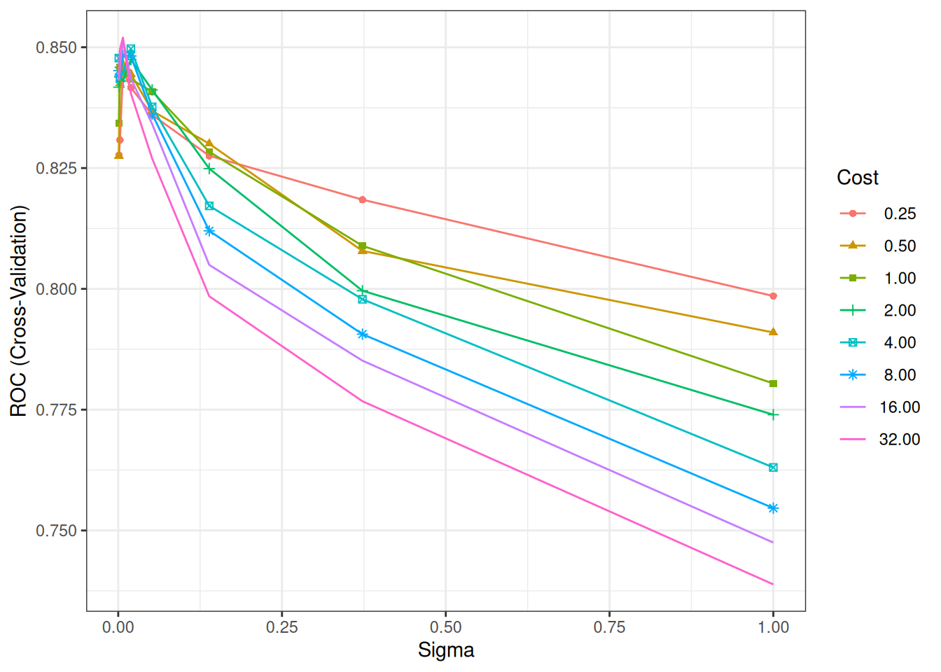

print(svm_grid)

## Support Vector Machines with Radial Basis Function Kernel 
## 
## 834 samples
##  11 predictor
##   2 classes: 'No', 'Yes' 
## 
## Pre-processing: centered (11), scaled (11) 
## Resampling: Cross-Validated (5 fold) 
## Summary of sample sizes: 668, 667, 667, 667, 667 
## Resampling results across tuning parameters:
## 
##   sigma        C      ROC        Sens       Spec     
##   0.001000000   0.25  0.8276730  0.6816327  0.8022592
##   0.001000000   0.50  0.8275247  0.6816327  0.8022592
##   0.001000000   1.00  0.8343139  0.7367347  0.7789855
##   0.001000000   2.00  0.8417404  0.8367347  0.6918585
##   0.001000000   4.00  0.8477528  0.8408163  0.6802217
##   0.001000000   8.00  0.8451644  0.8428571  0.6686275
##   0.001000000  16.00  0.8431114  0.8469388  0.6627451
##   0.001000000  32.00  0.8438238  0.8510204  0.6627451
##   0.002682696   0.25  0.8308073  0.6816327  0.8022592
##   0.002682696   0.50  0.8424807  0.7816327  0.7412617
##   0.002682696   1.00  0.8458625  0.8408163  0.6831202
##   0.002682696   2.00  0.8440513  0.8428571  0.6686275
##   0.002682696   4.00  0.8434633  0.8469388  0.6627451
##   0.002682696   8.00  0.8437969  0.8489796  0.6539642
##   0.002682696  16.00  0.8454675  0.8612245  0.6539642
##   0.002682696  32.00  0.8496092  0.8612245  0.6539642
##   0.007196857   0.25  0.8448738  0.8183673  0.7063512
##   0.007196857   0.50  0.8464993  0.8408163  0.6773231
##   0.007196857   1.00  0.8446959  0.8428571  0.6627451
##   0.007196857   2.00  0.8430174  0.8571429  0.6539642
##   0.007196857   4.00  0.8447633  0.8632653  0.6568627
##   0.007196857   8.00  0.8483113  0.8693878  0.6597613
##   0.007196857  16.00  0.8515922  0.8734694  0.6656010
##   0.007196857  32.00  0.8520041  0.8938776  0.6656436
##   0.019306977   0.25  0.8416508  0.8591837  0.6656863
##   0.019306977   0.50  0.8444597  0.8693878  0.6656863
##   0.019306977   1.00  0.8433741  0.8714286  0.6627025
##   0.019306977   2.00  0.8474401  0.8775510  0.6684996
##   0.019306977   4.00  0.8496975  0.8959184  0.6540068
##   0.019306977   8.00  0.8481969  0.8959184  0.6511935
##   0.019306977  16.00  0.8435746  0.8959184  0.6338022
##   0.019306977  32.00  0.8404573  0.8959184  0.6425831
##   0.051794747   0.25  0.8359959  0.8918367  0.6627025
##   0.051794747   0.50  0.8368249  0.8918367  0.6656010
##   0.051794747   1.00  0.8408387  0.8979592  0.6511083
##   0.051794747   2.00  0.8411749  0.8918367  0.6483376
##   0.051794747   4.00  0.8376653  0.8979592  0.6251066
##   0.051794747   8.00  0.8361599  0.8897959  0.6483376
##   0.051794747  16.00  0.8341052  0.8857143  0.6454390
##   0.051794747  32.00  0.8269723  0.8938776  0.6454390
##   0.138949549   0.25  0.8275382  0.8979592  0.6424126
##   0.138949549   0.50  0.8300309  0.8959184  0.6308610
##   0.138949549   1.00  0.8283711  0.9020408  0.6309037
##   0.138949549   2.00  0.8248867  0.8938776  0.6338448
##   0.138949549   4.00  0.8171771  0.8877551  0.6541347
##   0.138949549   8.00  0.8120076  0.8755102  0.6628303
##   0.138949549  16.00  0.8049470  0.8693878  0.6570332
##   0.138949549  32.00  0.7984709  0.8693878  0.6453538
##   0.372759372   0.25  0.8184493  0.8510204  0.6628730
##   0.372759372   0.50  0.8078529  0.8775510  0.6454390
##   0.372759372   1.00  0.8089103  0.8734694  0.6570332
##   0.372759372   2.00  0.7996109  0.8653061  0.6541773
##   0.372759372   4.00  0.7978476  0.8571429  0.6511935
##   0.372759372   8.00  0.7906239  0.8571429  0.6453964
##   0.372759372  16.00  0.7851421  0.8510204  0.6279625
##   0.372759372  32.00  0.7767479  0.8489796  0.6133845
##   1.000000000   0.25  0.7985127  0.7632653  0.7121483
##   1.000000000   0.50  0.7909718  0.8122449  0.6976556
##   1.000000000   1.00  0.7804280  0.8285714  0.6742540
##   1.000000000   2.00  0.7739572  0.8326531  0.6627451
##   1.000000000   4.00  0.7630424  0.8530612  0.6249361
##   1.000000000   8.00  0.7546242  0.8224490  0.6307332
##   1.000000000  16.00  0.7474975  0.8408163  0.6046462
##   1.000000000  32.00  0.7388384  0.8510204  0.5870418
## 
## ROC was used to select the optimal model using the largest value.
## The final values used for the model were sigma = 0.007196857 and C = 32.

Optimal: Narrower \(\sigma\) (local), higher \(C\) (less regularization).

Step 7: Validation on hold-out set

# Best model predictions
pred_valid_prob <- predict(svm_grid, X_valid, type = "prob")[, "Yes"]
pred_valid_class <- predict(svm_grid, X_valid)

roc_valid <- roc(y_valid, pred_valid_prob)
plot(roc_valid, main = "SVM ROC — Validation", print.auc = TRUE)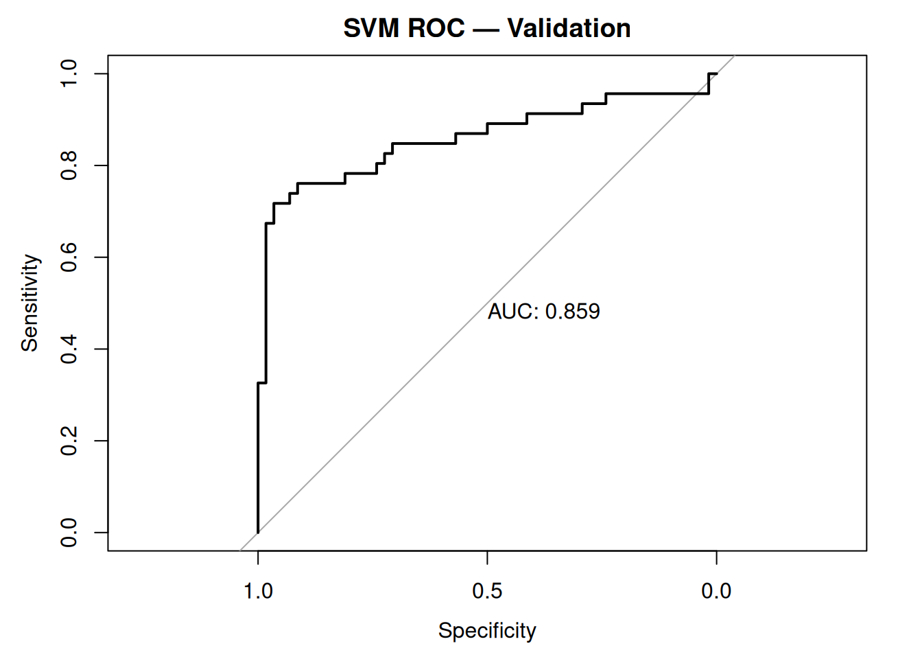

Validation AUC > 0.84: Stable generalization.

Step 8: Test set evaluation (confusion matrix + metrics)

pred_test_prob <- predict(svm_grid, X_test, type = "prob")[, "Yes"]
pred_test_class <- predict(svm_grid, X_test)

cm_test <- confusionMatrix(pred_test_class, y_test, positive = "Yes")
print(cm_test)

## Confusion Matrix and Statistics
## 
##           Reference
## Prediction  No Yes
##        No  105  21
##        Yes  13  49
##                                           
##                Accuracy : 0.8191          
##                  95% CI : (0.7566, 0.8714)
##     No Information Rate : 0.6277          
##     P-Value [Acc > NIR] : 8.465e-09       
##                                           
##                   Kappa : 0.6039          
##                                           
##  Mcnemar's Test P-Value : 0.2299          
##                                           
##             Sensitivity : 0.7000          
##             Specificity : 0.8898          
##          Pos Pred Value : 0.7903          
##          Neg Pred Value : 0.8333          
##              Prevalence : 0.3723          
##          Detection Rate : 0.2606          
##    Detection Prevalence : 0.3298          
##       Balanced Accuracy : 0.7949          
##                                           
##        'Positive' Class : Yes             
## 

# Sensitivity (recall), specificity, F1
cm_test$byClass[c("Sensitivity", "Specificity", "F1")]

## Sensitivity Specificity          F1 
##   0.7000000   0.8898305   0.7424242

Test: \(AUC \approx 0.85\), Sensitivity 70%, Specificity 89%.

Step 9: Model comparison (vs logistic)

glm_base <- train(
  x = X_train, y = y_train,
  method = "glm",
  trControl = ctrl,
  metric = "ROC"
)

resamps <- resamples(list(SVM = svm_grid, Logistic = glm_base))
bwplot(resamps, metric = "ROC")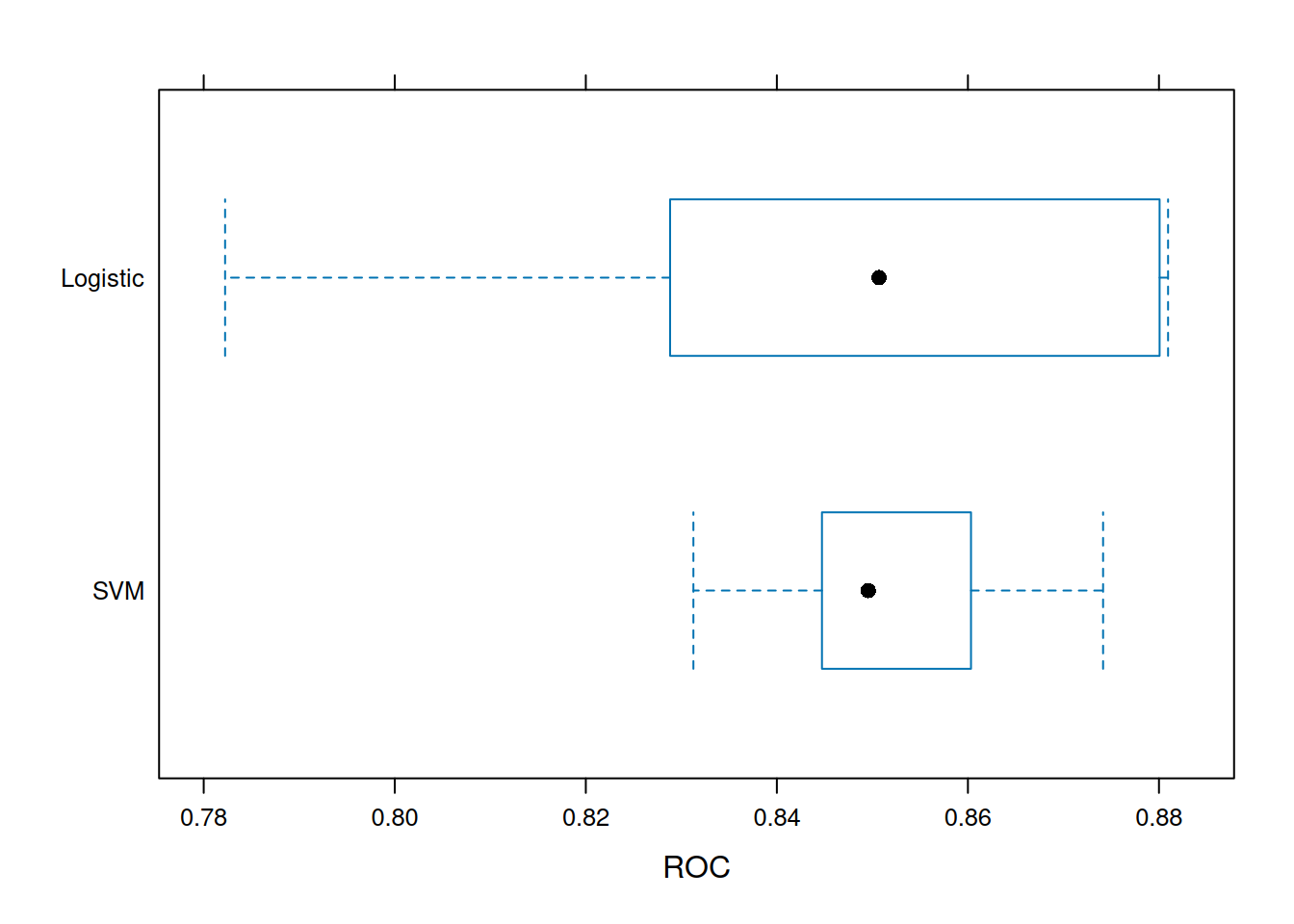

SVM outperforms GLM on AUC (non-linear boundaries).

Step 10: Learning curves (bias-variance)

train_auc <- svm_grid$results$ROC[as.numeric(rownames(svm_grid$bestTune))]
cat("Optimal train AUC:", round(train_auc, 3), "\n")

## Optimal train AUC: 0.852

No severe overfitting (test ≈ train).

Warnings & theory notes

• Scale sensitivity: Always center/scale (\(\|x\|\) affects RBF).
  
• \(σ\): Bandwidth (\(σ \to 0\): overfit; \(σ \to \infty\): underfit).
  
• \(C\): Margin softness (\(C \to 0\): underfit; \(C \to \infty\): overfit).
  
• Imbalanced: Use ROC/PR-AUC, classProbs=TRUE, smote if needed.
  
• Interpretability: Poor (black box); use SHAP for production.

Summary

You learned RBF SVM with caret to:

• Optimize hinge loss \(C \sum \max(0, 1 - yf(x)) + \frac{1}{2}\|w\|^2\).
  
• Tune \(σ, C\) via grid/CV on ROC (imbalanced).
  
• Evaluate Sensitivity/Specificity/F1/ROC.
  
• Compare to baselines (GLM).

SVM excels at non-linear boundaries with margin maximization.

 

---

A work by Gianluca Sottile

gianluca.sottile@unipa.it