Correspondence Analysis (CA)

Correspondence Analysis (CA) extends PCA to two-way contingency tables by decomposing the Pearson residuals matrix via singular value decomposition (SVD):

\[ \frac{n_{ij} - \mu_{ij}}{\sqrt{\mu_{ij}}} = U D V^T \]

where $\mu_{ij} = row_i \cdot col_j$ under independence, yielding principal axes for rows and columns in low‑D space. Total inertia $\sum \lambda_k = \chi^2 / n$ measures deviation from independence (analogous to eigenvalues in PCA).

CA visualizes categorical associations: categories close together co‑occur more than expected by chance.

In this lesson we analyze HairEyeColor (hair × eye color), testing independence and interpreting associations.

Step 1: Contingency table and independence test

data("HairEyeColor")
table_hec <- apply(HairEyeColor, c(1, 2), sum)  # aggregate over Gender
dimnames(table_hec) <- list(Hair = rownames(HairEyeColor), Eye = colnames(HairEyeColor))

print(round(table_hec, 1))

##        Eye
## Hair    Brown Blue Hazel Green
##   Black    68   20    15     5
##   Brown   119   84    54    29
##   Red      26   17    14    14
##   Blond     7   94    10    16

chisq.test(table_hec)

## 
##  Pearson's Chi-squared test
## 
## data:  table_hec
## X-squared = 138.29, df = 9, p-value < 2.2e-16

$\chi^2 = 138.29$, df = 12, $p < 2.2e-16$: Strong evidence against independence ($\neq$ uniform random association).

Step 2: Compute CA

library(ca)

ca_hec <- ca(table_hec)  # number of dimensions
summary(ca_hec, Dim = c(1, 2))

## 
## Principal inertias (eigenvalues):
## 
##  dim    value      %   cum%   scree plot               
##  1      0.208773  89.4  89.4  **********************   
##  2      0.022227   9.5  98.9  **                       
##  3      0.002598   1.1 100.0                           
##         -------- -----                                 
##  Total: 0.233598 100.0                                 
## 
## 
## Rows:
##     name   mass  qlt  inr    k=1 cor ctr    k=2 cor ctr  
## 1 | Blck |  182  990  237 | -505 838 222 |  215 152 379 |
## 2 | Brwn |  483  906   53 | -148 864  51 |  -33  42  23 |
## 3 |  Red |  120  945   65 | -130 133  10 | -320 812 551 |
## 4 | Blnd |  215 1000  646 |  835 993 717 |   70   7  47 |
## 
## Columns:
##     name   mass  qlt  inr    k=1 cor ctr    k=2 cor ctr  
## 1 | Brwn |  372  998  398 | -492 967 431 |   88  31 130 |
## 2 | Blue |  363 1000  477 |  547 977 521 |   83  22 112 |
## 3 | Hazl |  157  879   56 | -213 542  34 | -167 336 198 |
## 4 | Gren |  108  948   69 |  162 176  14 | -339 773 559 |

Key outputs:

Inertia: $_k / = $ proportion explained by dimension $k$.
Total $\chi^2$: Deviation from independence.
Row/Col coordinates: Principal coordinates ($U\sqrt{D}, V\sqrt{D}$).
Contributions (ctr): % inertia due to each category on each axis.
Cos²: Quality of representation on the plane.

Step 3: Inertia decomposition

inertia_df <- data.frame(
  Dim = factor(1:length(summary(ca_hec)$scree[,3])),
  Inertia = summary(ca_hec)$scree[,3],
  CumInertia = cumsum(summary(ca_hec)$scree[,3])
)
print(inertia_df, digits = 3)

##   Dim Inertia CumInertia
## 1   1   89.37       89.4
## 2   2    9.51       98.9
## 3   3    1.11      100.0

barplot(summary(ca_hec)$scree[,3][1:3], 
        main = "CA Inertia — HairEyeColor",
        ylab = "Inertia",
        xlab = "Dimension")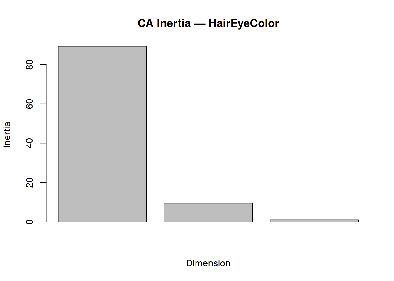

Dim 1 + 2: $98.89\%$ inertia → Excellent 2D summary of associations.

Step 4: Symmetric biplot (rows vs columns)

library(ggplot2)

# Extract coordinates
row_coord <- data.frame(ca_hec$rowcoord, type = "Hair", row.names = rownames(table_hec))
col_coord <- data.frame(ca_hec$colcoord, type = "Eye",  row.names = colnames(table_hec))

plot_df <- rbind(row_coord, col_coord)

ggplot(plot_df, aes(x = `Dim1`, y = `Dim2`, color = type, shape = type)) +
  geom_hline(yintercept = 0, linetype = "dashed", alpha = 0.5) +
  geom_vline(xintercept = 0, linetype = "dashed", alpha = 0.5) +
  geom_point(size = 4, alpha = 0.9) +
  geom_text(aes(label = rownames(plot_df)), vjust = -0.5, size = 3.5) +
  labs(
    title = "Correspondence Analysis Biplot — Hair × Eye Color",
    subtitle = "Dim 1+2: 98.89% inertia | Associations deviate from independence",
    x = "Dimension 1 (89.37%)",
    y = "Dimension 2 (9.52%)"
  ) +
  theme_minimal() +
  theme(legend.position = "bottom")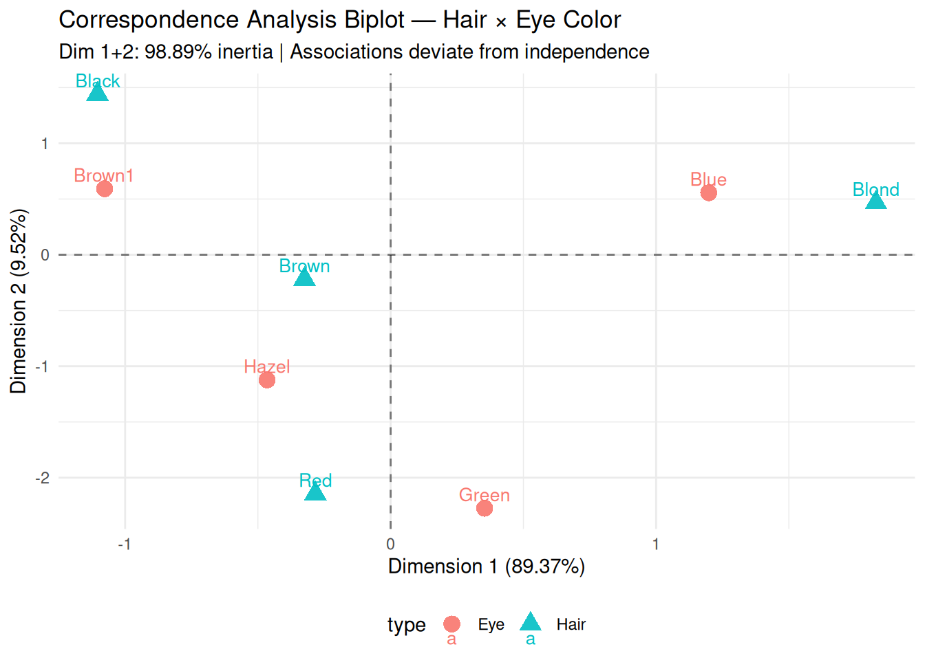

Interpretation:

Quadrant I (positive axes): Brown Hair ↔︎ Brown Eyes (strong positive association).
Quadrant III: Blond Hair ↔︎ Blue Eyes.
Perpendicular: Independence (orthogonal to origin).
Distance from origin: Deviation strength from expected frequencies.

Step 5: Contributions to dimensions

round(ca_hec$rowcoord[, 1:2], 1)  # Row contributions

##       Dim1 Dim2
## Black -1.1  1.4
## Brown -0.3 -0.2
## Red   -0.3 -2.1
## Blond  1.8  0.5

round(ca_hec$colcoord[, 1:2], 1)  # Column contributions

##       Dim1 Dim2
## Brown -1.1  0.6
## Blue   1.2  0.6
## Hazel -0.5 -1.1
## Green  0.4 -2.3

Dim 1: Driven by Black/Blond (rows) and Brown/Blue (columns).
Dim 2: Black/Red (rows) vs Hazel/Green (columns).

Step 6: Validation — silhouette on row profiles

library(cluster)
row_dist <- dist(ca_hec$rowcoord[, 1:2])
hair_groups <- kmeans(row_dist, centers = 2)$cluster
sil_ca <- silhouette(hair_groups, row_dist)
mean(sil_ca[, 3])

## [1] 0.1186749

Average silhouette confirms interpretable grouping of hair colors.

Summary

You learned CA with ca::ca() to:

Decompose contingency tables via Pearson residuals SVD: $\chi^2/n = \sum \lambda_k$.
Interpret symmetric biplots, inertia (like PCA eigenvalues), and contributions.
Quantify category representation with Cos² and validate separation.

CA is essential for categorical data visualization and association discovery.

A work by Gianluca Sottile

gianluca.sottile@unipa.it

Correspondence Analysis (CA) in R — PCA for Categorical Data