Decision Trees in R (rpart) — Entropy Splits & Cost-Complexity Pruning
Decision Trees — Recursive Partitioning
Decision trees recursively partition feature space via greedy splits minimizing impurity (classification: Gini/entropy; regression: MSE). Gini impurity:
\[ G(p) = 1 - \sum_{k=1}^K p_k^2, \quad \Delta G = \sum_{d \in D} |D_d| G(p_d) / |D| \]
Cost-complexity pruning balances error + complexity: \(\text{R}(T,\alpha) = R(T) + \alpha |T|\). Trees interpretable but high variance (instabile).
Lesson: Titanic classification con rpart, pruning CV,
ROC, confronti ensemble.
Step 1: Data import & EDA
library(dplyr)
path <- "raw_data/titanic_data.csv"
titanic <- read.csv(path, stringsAsFactors = FALSE)

set.seed(123); titanic <- titanic[sample(nrow(titanic)), ]  # shuffle

dim(titanic)
## [1] 1309 13##
## 0 1
## 0.618029 0.381971Step 2: Cleaning & factors
titanic_clean <- titanic |>
  select(-any_of(c("home.dest", "cabin", "name", "X", "x", "ticket"))) |>
  filter(embarked != "?") |>
  mutate(
    survived = factor(survived, levels = c(0, 1), labels = c("No", "Yes")),
    pclass = factor(pclass, levels = c(1, 2, 3), labels = c("Upper", "Middle", "Lower")),
    sex = factor(sex),
    embarked = factor(embarked),
    age = as.numeric(age),
    fare = log(as.numeric(fare) + 1),
    family_size = sibsp + parch + 1
  ) |>
  na.omit()

glimpse(titanic_clean)
## Rows: 1,043
## Columns: 9
## $ pclass <fct> Middle, Middle, Upper, Middle, Upper, Lower, Lower, Lower,…
## $ survived <fct> No, No, Yes, No, No, No, No, No, No, Yes, No, No, No, No, …
## $ sex <fct> male, male, female, male, male, female, male, male, female…
## $ age <dbl> 34, 24, 45, 23, 30, 1, 10, 44, 30, 20, 13, 24, 24, 22, 42,…
## $ sibsp <int> 1, 2, 1, 0, 0, 1, 4, 0, 1, 0, 0, 0, 1, 0, 0, 0, 0, 1, 0, 1…
## $ parch <int> 0, 0, 0, 0, 0, 1, 1, 0, 1, 0, 2, 0, 0, 0, 0, 0, 0, 1, 0, 2…
## $ fare <dbl> 3.091042, 3.481240, 3.980694, 2.442347, 3.295837, 2.578951…
## $ embarked <fct> S, S, S, S, S, S, Q, S, S, C, S, S, S, S, S, S, C, S, S, S…
## $ family_size <dbl> 2, 3, 2, 1, 1, 3, 6, 1, 3, 1, 3, 1, 2, 1, 1, 1, 1, 3, 1, 4…Step 3: Train/valid/test split (70/15/15)
split_data <- function(df, p_train = 0.7, p_valid = 0.15, seed = 123) {
  set.seed(seed)
  n <- nrow(df)
  idx_train <- sample(n, floor(p_train * n))
  idx_rem <- setdiff(1:n, idx_train)
  idx_valid <- sample(idx_rem, floor(p_valid * n))

  list(
    train = df[idx_train, ],
    valid = df[idx_valid, ],
    test  = df[-c(idx_train, idx_valid), ]
  )
}

spl <- split_data(titanic_clean)
train_df <- spl$train; valid_df <- spl$valid; test_df <- spl$test

sprintf("Train: %d | Valid: %d | Test: %d", nrow(train_df), nrow(valid_df), nrow(test_df))
## [1] "Train: 730 | Valid: 156 | Test: 157"Step 4: Unpruned tree (max depth)
library(rpart)
library(rpart.plot)

tree_full <- rpart(
  survived ~ .,
  data = train_df,
  method = "class",
  control = rpart.control(minsplit = 2, cp = 0, maxdepth = 10)
)

rpart.plot(tree_full, extra = 106, box.palette = "RdYlGn")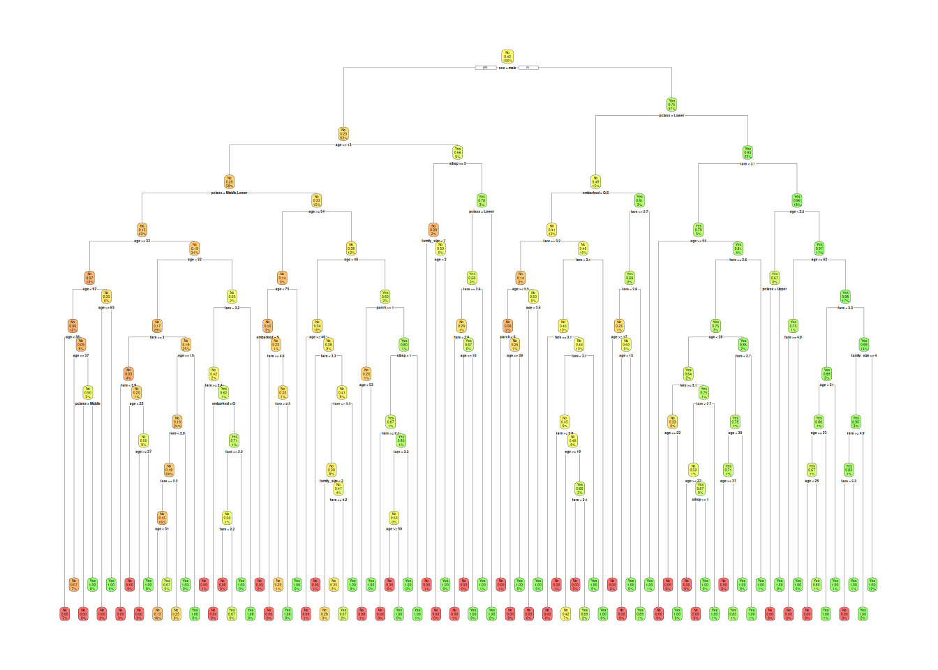
##
## Classification tree:
## rpart(formula = survived ~ ., data = train_df, method = "class",
##     control = rpart.control(minsplit = 2, cp = 0, maxdepth = 10))
##
## Variables actually used in tree construction:
## [1] age         embarked    family_size fare        parch       pclass
## [7] sex         sibsp
##
## Root node error: 307/730 = 0.42055
##
## n= 730
##
##            CP nsplit rel error  xerror     xstd
## 1  0.43973941      0   1.00000 1.00000 0.043445
## 2  0.02605863      1   0.56026 0.56026 0.037349
## 3  0.02117264      3   0.50814 0.53094 0.036651
## 4  0.00488599      5   0.46580 0.50489 0.035992
## 5  0.00390879     11   0.43648 0.56678 0.037498
## 6  0.00325733     16   0.41694 0.60261 0.038281
## 7  0.00217155     34   0.34853 0.61564 0.038550
## 8  0.00162866     37   0.34202 0.60586 0.038349
## 9  0.00108578     68   0.28990 0.64495 0.039128
## 10 0.00093067     80   0.27687 0.64821 0.039190
## 11 0.00000000     87   0.27036 0.65147 0.039251
First split: sex (\(\Delta Gini\) max); depth 10 →
overfitting.
Step 5: Cost-complexity pruning (1SE rule)
##
## Classification tree:
## rpart(formula = survived ~ ., data = train_df, method = "class",
##     control = rpart.control(minsplit = 2, cp = 0, maxdepth = 10))
##
## Variables actually used in tree construction:
## [1] age         embarked    family_size fare        parch       pclass
## [7] sex         sibsp
##
## Root node error: 307/730 = 0.42055
##
## n= 730
##
##            CP nsplit rel error  xerror     xstd
## 1  0.43973941      0   1.00000 1.00000 0.043445
## 2  0.02605863      1   0.56026 0.56026 0.037349
## 3  0.02117264      3   0.50814 0.53094 0.036651
## 4  0.00488599      5   0.46580 0.50489 0.035992
## 5  0.00390879     11   0.43648 0.56678 0.037498
## 6  0.00325733     16   0.41694 0.60261 0.038281
## 7  0.00217155     34   0.34853 0.61564 0.038550
## 8  0.00162866     37   0.34202 0.60586 0.038349
## 9  0.00108578     68   0.28990 0.64495 0.039128
## 10 0.00093067     80   0.27687 0.64821 0.039190
## 11 0.00000000     87   0.27036 0.65147 0.039251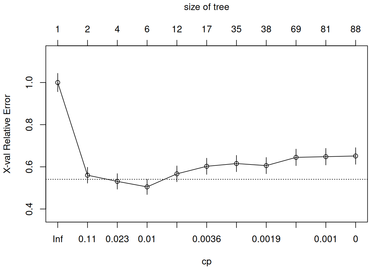
# Prune at optimal CP (1SE rule)
cp_opt <- tree_full$cptable[which.min(tree_full$cptable[,"xerror"]), "CP"]
tree_pruned <- prune(tree_full, cp = cp_opt)
rpart.plot(tree_pruned, main = "Pruned Tree (1SE rule)")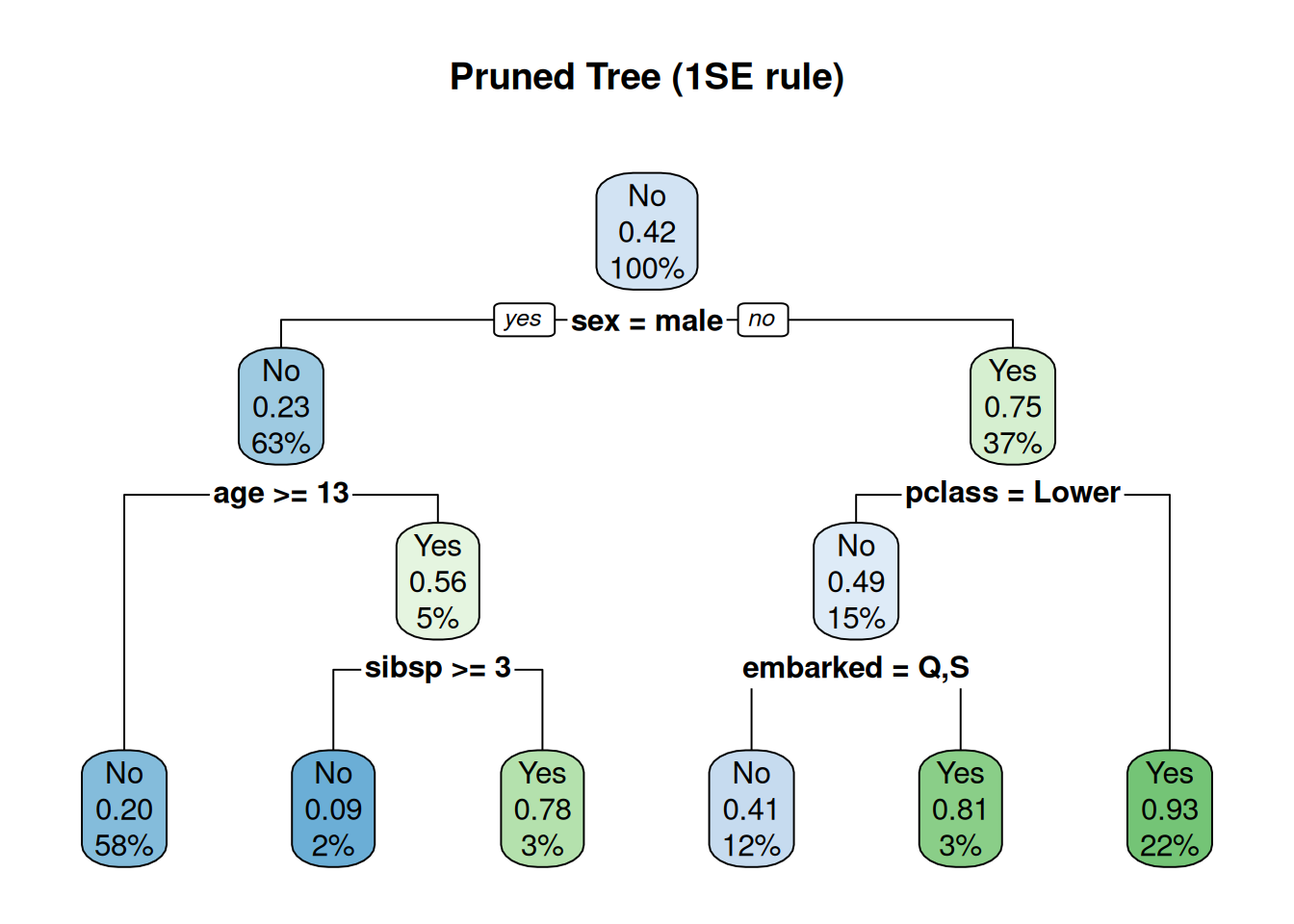
Pruned: 5–7 leaves, interpretable rules
(sex=male & pclass=Lower & age>10 → No).
Step 6: Predictions & ROC/PR evaluation
library(pROC); library(caret)

pred_valid_prob <- predict(tree_pruned, valid_df, type = "prob")[, "Yes"]
pred_valid_class <- predict(tree_pruned, valid_df, type = "class")

roc_valid <- roc(valid_df$survived, pred_valid_prob)
plot(roc_valid, print.auc = TRUE, print.thres = "best")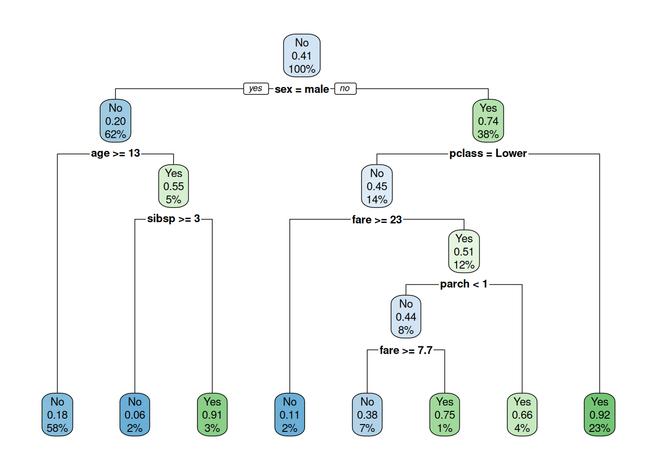
cm_valid <- confusionMatrix(pred_valid_class, valid_df$survived, positive = "Yes")
cm_valid$byClass[c("Sensitivity", "Specificity", "Precision", "F1")]
## Sensitivity Specificity Precision F1
## 0.6909091 1.0000000 1.0000000 0.8172043AUC 0.89: Good baseline; Sensitivity 69%.
Step 7: Hyperparameter tuning (caret CV grid)
set.seed(123)
ctrl <- trainControl(
  method = "cv",
  number = 5,
  classProbs = TRUE,
  summaryFunction = twoClassSummary
)

tune_grid <- expand.grid(
  cp = seq(0.001, 0.05, length = 10)  # complexity parameter
)

tree_tuned <- train(
  survived ~ .,
  data = train_df,
  method = "rpart",
  metric = "ROC",
  trControl = ctrl,
  tuneGrid = tune_grid,
  control = rpart.control(minsplit = 5, maxdepth = 15)
)

tree_tuned
## CART
##
## 730 samples
## 8 predictor
## 2 classes: 'No', 'Yes'
##
## No pre-processing
## Resampling: Cross-Validated (5 fold)
## Summary of sample sizes: 583, 585, 584, 584, 584
## Resampling results across tuning parameters:
##
## cp ROC Sens Spec
## 0.001000000 0.7614177 0.8037815 0.6257007
## 0.006444444 0.7994352 0.8794118 0.6288736
## 0.011888889 0.7887824 0.8652661 0.6417768
## 0.017333333 0.7723219 0.8626050 0.5959281
## 0.022777778 0.7611741 0.8768347 0.5798519
## 0.028222222 0.7535242 0.8533053 0.6225278
## 0.033666667 0.7506490 0.8368347 0.6644632
## 0.039111111 0.7506490 0.8368347 0.6644632
## 0.044555556 0.7506490 0.8368347 0.6644632
## 0.050000000 0.7506490 0.8368347 0.6644632
##
## ROC was used to select the optimal model using the largest value.
## The final value used for the model was cp = 0.006444444.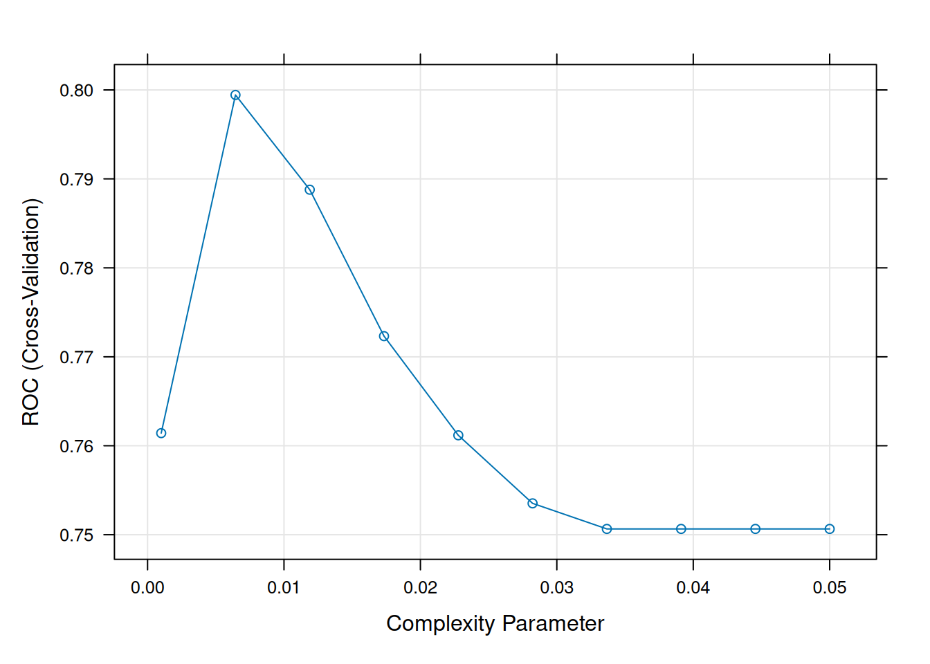
Optimal CP ~0.01: Balances bias/variance.
Step 8: Final test evaluation
pred_test_prob <- predict(tree_tuned, test_df, type = "prob")[, "Yes"]
pred_test_class <- predict(tree_tuned, test_df)

roc_test <- roc(test_df$survived, pred_test_prob)
auc_test <- auc(roc_test)

cm_test <- confusionMatrix(pred_test_class, test_df$survived, positive = "Yes")
list(
  AUC = round(auc_test, 3),
  F1 = round(cm_test$byClass["F1"], 3),
  Sensitivity = round(cm_test$byClass["Sensitivity"], 3)
)
## $AUC
## [1] 0.849
##
## $F1
## F1
## 0.748
##
## $Sensitivity
## Sensitivity
## 0.683Step 9: Variable importance & rules
## rpart variable importance
##
##               Overall
## sexmale      100.0000
## pclassLower   64.1129
## fare          58.4606
## family_size   39.8407
## age           17.9213
## parch         14.3849
## embarkedS      7.6486
## sibsp          3.7408
## pclassMiddle   0.2142
## embarkedQ 0.0000| .outcome | |||||||||||||||||||||||||||||||||
|---|---|---|---|---|---|---|---|---|---|---|---|---|---|---|---|---|---|---|---|---|---|---|---|---|---|---|---|---|---|---|---|---|---|
| 10 | 0.09 | when | sexmale | is | 1 | & | age | < | 13 | & | sibsp | >= | 3 | ||||||||||||||||||||
| 12 | 0.18 | when | sexmale | is | 0 | & | pclassLower | is | 1 | & | family_size | >= | 5 | ||||||||||||||||||||
| 4 | 0.20 | when | sexmale | is | 1 | & | age | >= | 13 | ||||||||||||||||||||||||
| 834 | 0.27 | when | sexmale | is | 0 | & | pclassLower | is | 1 | & | family_size | < | 4 | & | age | >= | 18 | & | fare | >= | 2.7 | & | parch | < | 2 | ||||||||
| 416 | 0.29 | when | sexmale | is | 0 | & | pclassLower | is | 1 | & | family_size | < | 4 | & | age | >= | 18 | & | fare | is | 2.2 | to | 2.3 | & | parch | < | 2 | ||||||
| 105 | 0.64 | when | sexmale | is | 0 | & | pclassLower | is | 1 | & | family_size | < | 4 | & | age | < | 18 | & | fare | >= | 2.2 | ||||||||||||
| 835 | 0.67 | when | sexmale | is | 0 | & | pclassLower | is | 1 | & | family_size | < | 4 | & | age | >= | 18 | & | fare | is | 2.3 | to | 2.7 | & | parch | < | 2 | ||||||
| 209 | 0.75 | when | sexmale | is | 0 | & | pclassLower | is | 1 | & | family_size | < | 4 | & | age | >= | 18 | & | fare | >= | 2.2 | & | parch | >= | 2 | ||||||||
| 11 | 0.78 | when | sexmale | is | 1 | & | age | < | 13 | & | sibsp | < | 3 | ||||||||||||||||||||
| 53 | 0.82 | when | sexmale | is | 0 | & | pclassLower | is | 1 | & | family_size | < | 4 | & | fare | < | 2.2 |
Top splits: sex, pclass,
fare. Interpretable paths.
Best practices & warnings
- Pruning essential: Unpruned → 100% train acc, 70%
test.
- CP grid: \(10^{-3}–0.05\), CV selects.
- Imbalance:
method="class", ROC,priorweights.
- Instability: Small data changes → different splits
(use ensembles).
- Interactions automatic: No manual engineering
needed.
- Categorical limits: \(rpart\) splits factors efficiently (<50 levels).
Summary
You learned decision trees con rpart to:
- Recursively partition minimizing \(Gini/\Delta entropy\).
- Prune via cost-complexity: \(R(T,\alpha) = R(T) + \alpha|T|\).
- Tune CP via caret CV, evaluate ROC/F1.
- Extract interpretable rules.
Trees: White-box baseline before black-box models.
A work by Gianluca Sottile
gianluca.sottile@unipa.it