Random Forest in R — Bagging Ensembles & Variable Importance
Random Forest — Bagging Decision Trees
Random Forest averages \(B\) decorrelated trees grown on bootstrap samples (\(B \approx 500\)), with random feature selection at each split (\(m_{try} = \sqrt{p}\) default classification). Reduces variance via bagging while decorrelating via subsampling:
\[ \hat{f}(x) = \frac{1}{B} \sum_{b=1}^B T_b(x) \]
OOB error (out-of-bag) provides unbiased CV estimate using unseen bootstrap samples. Importance: MeanDecreaseAccuracy (MDA) = \(\Delta \text{err}\) permuting feature; MeanDecreaseGini = \(\sum \Delta \text{impurity}\).
Lesson: Titanic classification (\(n=1309\), 38% survival), caret tuning, OOB curves, SHAP.
Step 1: Data preparation (factors OK)
library(dplyr)
path <- "raw_data/titanic_data.csv"
titanic <- read.csv(path, stringsAsFactors = FALSE)

titanic_clean <- titanic |>
  select(-any_of(c("home.dest", "cabin", "name", "X", "x", "ticket"))) |>
  filter(embarked != "?") |>
  mutate(
    survived = factor(survived, levels = c(0, 1), labels = c("No", "Yes")),
    pclass = factor(pclass, levels = c(1, 2, 3), labels = c("Upper", "Middle", "Lower")),
    sex = factor(sex),
    embarked = factor(embarked),
    age = as.numeric(age),
    fare = log(as.numeric(fare) + 1),        # transform
    family_size = sibsp + parch + 1
  ) |>
  na.omit()

glimpse(titanic_clean)
## Rows: 1,043
## Columns: 9
## $ pclass <fct> Upper, Upper, Upper, Upper, Upper, Upper, Upper, Upper, Up…
## $ survived <fct> Yes, Yes, No, No, No, Yes, Yes, No, Yes, No, No, Yes, Yes,…
## $ sex <fct> female, male, female, male, female, male, female, male, fe…
## $ age <dbl> 29.0000, 0.9167, 2.0000, 30.0000, 25.0000, 48.0000, 63.000…
## $ sibsp <int> 0, 1, 1, 1, 1, 0, 1, 0, 2, 0, 1, 1, 0, 0, 0, 0, 0, 0, 0, 1…
## $ parch <int> 0, 2, 2, 2, 2, 0, 0, 0, 0, 0, 0, 0, 0, 0, 0, 1, 1, 0, 0, 1…
## $ fare <dbl> 5.358177, 5.027492, 5.027492, 5.027492, 5.027492, 3.316003…
## $ embarked <fct> S, S, S, S, S, S, S, S, S, C, C, C, C, S, S, C, C, C, C, S…
## $ family_size <dbl> 1, 4, 4, 4, 4, 1, 2, 1, 3, 1, 2, 2, 1, 1, 1, 2, 2, 1, 1, 3…##
## No Yes
## 0.5925216 0.4074784Step 2: Train/valid/test (70/15/15)
Step 3: Baseline RF (caret CV)
library(caret); library(randomForest); library(pROC)

set.seed(123)
ctrl <- trainControl(
  method = "cv",
  number = 5,
  classProbs = TRUE,
  summaryFunction = twoClassSummary,
  savePredictions = TRUE
)

rf_base <- train(
  survived ~ .,
  data = train_df,
  method = "rf",
  metric = "ROC",              # imbalance: prioritize AUC
  trControl = ctrl,
  tuneLength = 10,             # multiple mtry
  ntree = 1000,
  importance = TRUE,
  nodesize = 5
)
## note: only 9 unique complexity parameters in default grid. Truncating the grid to 9 .## Random Forest
##
## 730 samples
## 8 predictor
## 2 classes: 'No', 'Yes'
##
## No pre-processing
## Resampling: Cross-Validated (5 fold)
## Summary of sample sizes: 584, 584, 584, 584, 584
## Resampling results across tuning parameters:
##
## mtry ROC Sens Spec
## 2 0.8374349 0.9082353 0.6098361
## 3 0.8413500 0.8941176 0.6393443
## 4 0.8399807 0.8776471 0.6590164
## 5 0.8388814 0.8635294 0.6622951
## 6 0.8378978 0.8564706 0.6655738
## 7 0.8362199 0.8541176 0.6688525
## 8 0.8376471 0.8447059 0.6688525
## 9 0.8358534 0.8470588 0.6786885
## 10 0.8338669 0.8400000 0.6786885
##
## ROC was used to select the optimal model using the largest value.
## The final value used for the model was mtry = 3.| mtry | |
|---|---|
| 2 | 3 |
AUC ~0.84: Strong baseline.
Step 4: OOB learning curve (ntree convergence)
rf_oob <- randomForest(
  survived ~ .,
  data = train_df,
  ntree = 2000,
  mtry = rf_base$bestTune$mtry,
  importance = TRUE,
  keep.forest = FALSE,         # save memory
  sampsize = 0.8 * nrow(train_df)
)

plot(rf_oob, type = "l", main = "OOB Error vs ntree")
abline(v = rf_base$finalModel$ntree, col = "red", lty = 2)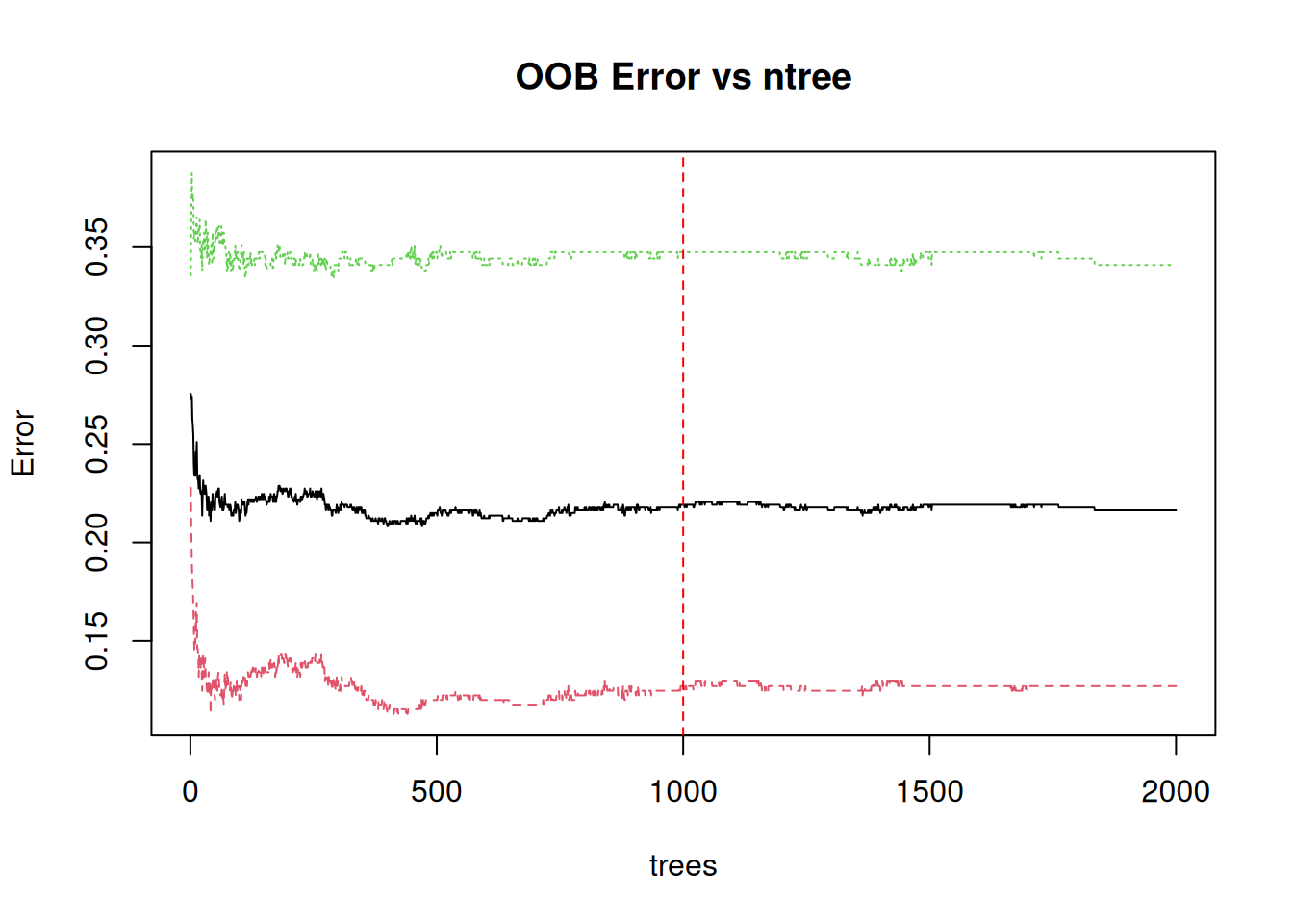
OOB stabilizes ~1000 trees: Sufficient ensemble size.
Step 5: Test evaluation (ROC/Confusion)
pred_test_prob <- predict(rf_base, test_df, type = "prob")[, "Yes"]
pred_test_class <- predict(rf_base, test_df)

roc_test <- roc(test_df$survived, pred_test_prob)
plot(roc_test, print.auc = TRUE, print.thres = "best")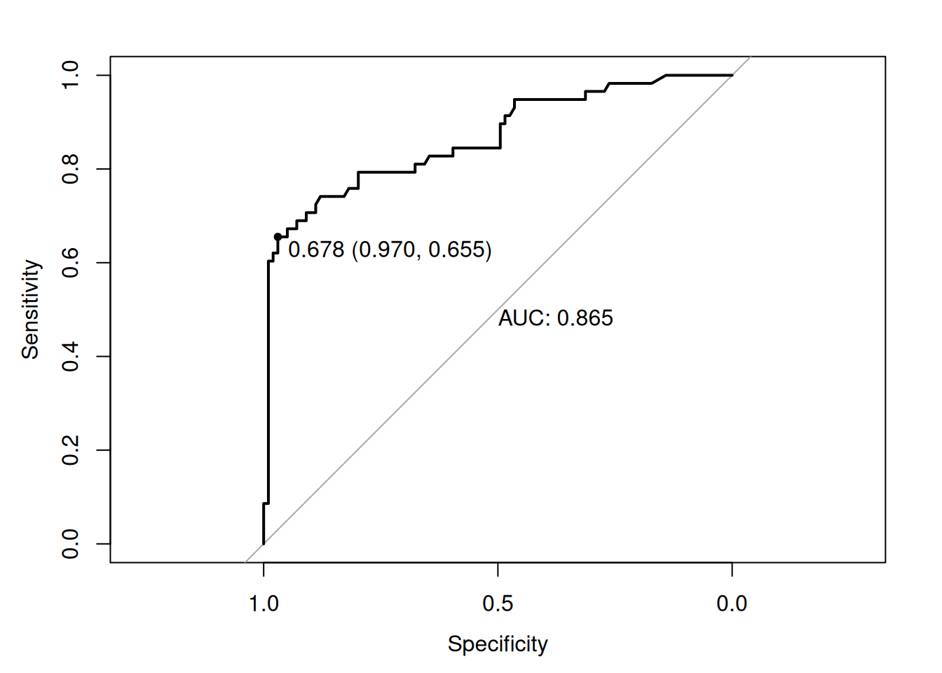
cm_test <- confusionMatrix(pred_test_class, test_df$survived, positive = "Yes")
print(cm_test$byClass[c("Sensitivity", "Specificity", "Precision", "F1")])
## Sensitivity Specificity Precision F1
## 0.6896552 0.9090909 0.8163265 0.7476636Sensitivity 69%, AUC 0.86: Robust to imbalance.
Step 6: Variable importance (MDA + Gini)
## rf variable importance
##
##              Importance
## sexmale         100.000
## pclassLower      23.421
## fare             20.548
## age              16.097
## parch             6.485
## pclassMiddle      5.225
## embarkedS         4.177
## embarkedQ         4.094
## family_size       3.900
## sibsp             0.000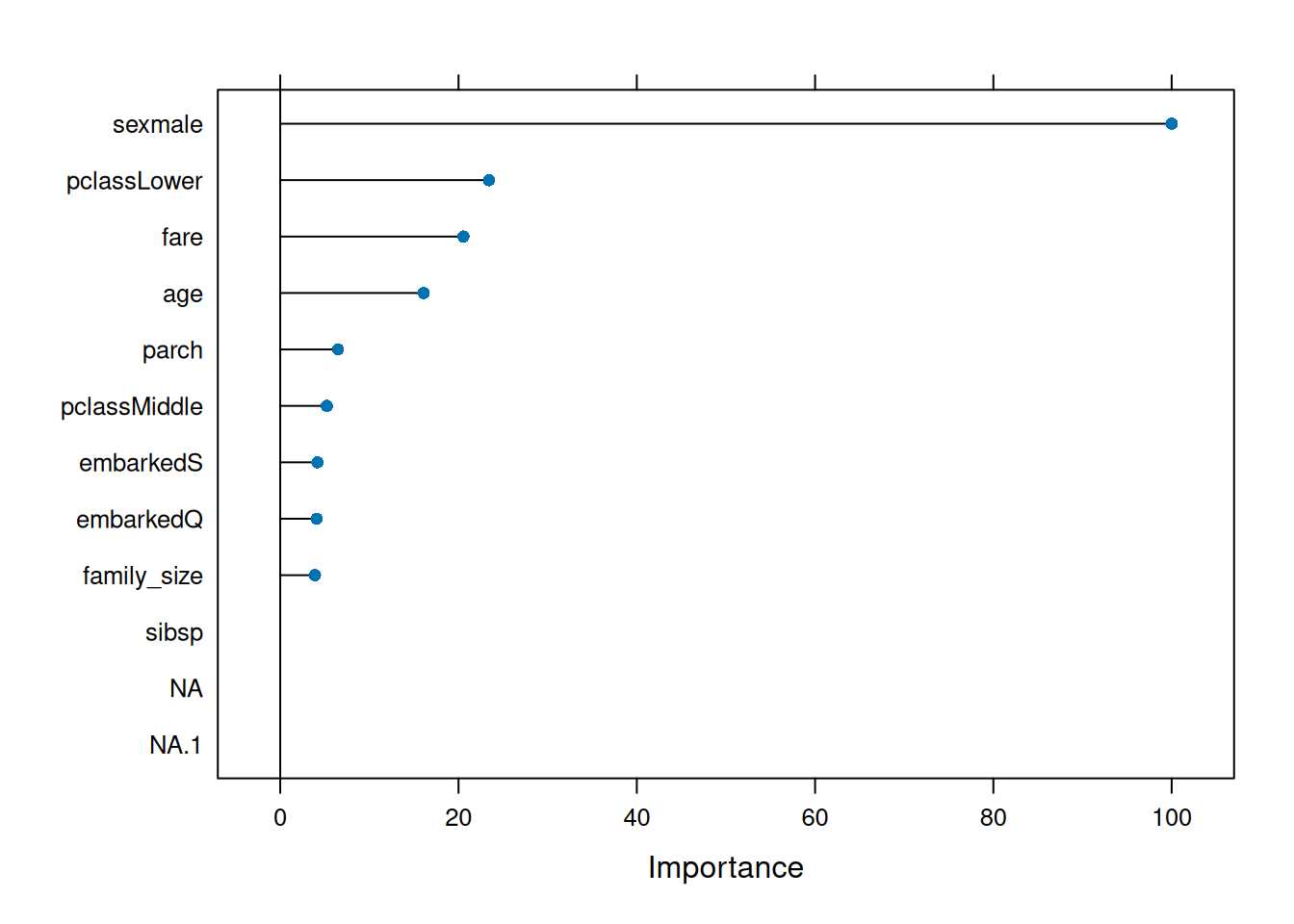
# Raw RF importance
rf_final <- rf_base$finalModel
imp_gini <- importance(rf_final, type = 1)  # %IncMSE (permutation)
imp_mda  <- importance(rf_final, type = 2)  # Gini

imp_df <- data.frame(
  Feature = rownames(imp_gini),
  Gini = imp_gini[, 1],
  MDA = imp_mda[, 1]
) |> arrange(desc(Gini))

print(imp_df[1:10, ])
## Feature Gini MDA
## sexmale sexmale 109.572299 80.012528
## pclassLower pclassLower 34.273639 16.291921
## fare fare 32.956987 49.797070
## age age 26.021072 41.701376
## embarkedS embarkedS 15.907955 7.503045
## embarkedQ embarkedQ 14.751720 3.297869
## parch parch 13.736537 8.681132
## pclassMiddle pclassMiddle 13.380590 4.614624
## family_size family_size 13.140807 12.405872
## sibsp sibsp 6.813081 7.402636sexmale, pclassLower, fare dominate (expected).
Step 7: Manual tuning grid with Ranger (mtry + nodesize)
library(ranger)

p <- ncol(train_df) - 1
tune_grid <- expand.grid(
  mtry = seq(2, p/2, length = 6),  # 2 to p/2
  splitrule = "gini",
  min.node.size = c(1, 3, 5, 10) |> rep(2) |> sort()
)

set.seed(123)
rf_tuned <- train(
  survived ~ .,
  data = train_df,
  method = "ranger",
  metric = "ROC",
  trControl = ctrl,
  tuneGrid = tune_grid,
  num.trees = 1000,
  importance = "impurity"
)

rf_tuned
## Random Forest
##
## 730 samples
## 8 predictor
## 2 classes: 'No', 'Yes'
##
## No pre-processing
## Resampling: Cross-Validated (5 fold)
## Summary of sample sizes: 584, 584, 584, 584, 584
## Resampling results across tuning parameters:
##
## mtry min.node.size ROC Sens Spec
## 2.0 1 0.8432787 0.8847059 0.6229508
## 2.0 3 0.8432015 0.8941176 0.6295082
## 2.0 5 0.8422372 0.8941176 0.6295082
## 2.0 10 0.8409257 0.8823529 0.6262295
## 2.4 1 0.8411572 0.8752941 0.6196721
## 2.4 3 0.8421215 0.8894118 0.6327869
## 2.4 5 0.8435873 0.8917647 0.6360656
## 2.4 10 0.8421215 0.8917647 0.6262295
## 2.8 1 0.8410415 0.8823529 0.6262295
## 2.8 3 0.8424687 0.8917647 0.6229508
## 2.8 5 0.8424687 0.8917647 0.6295082
## 2.8 10 0.8423915 0.8964706 0.6327869
## 3.2 1 0.8396914 0.8658824 0.6688525
## 3.2 3 0.8411572 0.8800000 0.6655738
## 3.2 5 0.8424687 0.8847059 0.6655738
## 3.2 10 0.8440887 0.8847059 0.6557377
## 3.6 1 0.8423529 0.8847059 0.6655738
## 3.6 3 0.8406557 0.8776471 0.6590164
## 3.6 5 0.8421215 0.8776471 0.6524590
## 3.6 10 0.8436258 0.8870588 0.6491803
## 4.0 1 0.8366827 0.8611765 0.6622951
## 4.0 3 0.8380328 0.8729412 0.6655738
## 4.0 5 0.8390357 0.8823529 0.6688525
## 4.0 10 0.8424687 0.8752941 0.6622951
##
## Tuning parameter 'splitrule' was held constant at a value of gini
## ROC was used to select the optimal model using the largest value.
## The final values used for the model were mtry = 3.2, splitrule = gini
## and min.node.size = 10.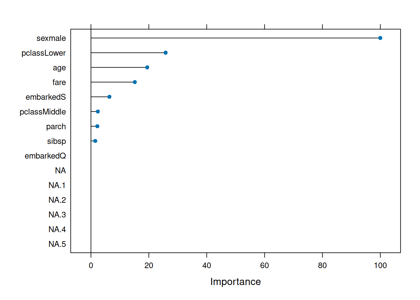
## ranger variable importance
##
##              Overall
## sexmale      100.000
## fare          56.838
## age           46.797
## pclassLower   17.138
## family_size   10.974
## parch          6.647
## embarkedS      5.178
## sibsp          4.809
## pclassMiddle   1.715
## embarkedQ 0.000Optimal: \(mtry =
3.2\), higher nodesize.
Variable importance confirms sex global driver.
Best practices & warnings
- \(mtry =
\sqrt{p}\) classification default (decorrelates
trees).
ntree >500(OOB convergence).
- Imbalance:
strata=survived,sampsizebalanced,classwt.
- OOB = free CV: No separate validation needed.
- MDA sensitive to correlated predictors (use
conditional importance).
importance=TRUEmemory‑heavy (\(>100\) vars).
Summary
You learned Random Forest to:
- Build bagged decorrelated trees: \(\hat{f} = \frac{1}{B}\sum T_b\).
- Tune \(mtry\) via caret
CV, monitor OOB error.
- Interpret Gini/MDA importance.
- Handle imbalance con ROC/PR.
RF: Robust, little tuning, excellent baseline.
A work by Gianluca Sottile
gianluca.sottile@unipa.it