Missing data
Find NAs, understand why they are missing, and handle them without fooling yourself
Locate missing values, learn the three missingness mechanisms (MCAR, MAR, MNAR) through a simulation, see when complete-case analysis is biased, and understand why mean imputation shrinks variability and distorts correlations; pointers to multiple imputation with mice.
NoteLearning objectives
By the end of this lesson you will be able to:
- find and count missing values in vectors and data frames;
- explain the three missingness mechanisms (MCAR, MAR, MNAR) with everyday examples;
- show by simulation when complete-case analysis gives biased results;
- remove or replace missing values with
na.rm,drop_na(),na.omit()andreplace_na(), knowing what each choice costs; - explain why mean imputation shrinks the variance and weakens correlations, and know that multiple imputation exists for serious work.
library(dplyr)
library(tidyr)
library(readr)
library(ggplot2)
1. Why missing data matter
Almost every real dataset has holes: a survey question left blank, a sensor that stopped recording, a patient who left a study. R marks a missing value with NA (“not available”).
Missing values cause two kinds of trouble:
- Technical: many functions return
NA, or fail, as soon as one value is missing. - Statistical: if the values are missing for a reason, the observed data are no longer a fair picture of the population, and simply ignoring the holes can give biased answers.
The first problem takes one argument to fix. The second needs thinking, and is the heart of this lesson.
2. NA in R
NA is contagious: any computation involving an unknown value gives an unknown result.
x <- c(12, NA, 7, 3)
mean(x)
#> [1] NAmean(x, na.rm = TRUE) # remove NAs before computing#> [1] 7.333sum(is.na(x)) # how many are missing?#> [1] 1You cannot test for NA with ==, because “is this unknown value equal to NA?” is itself unknown:
x == NA # all NA: not what you want#> [1] NA NA NA NAis.na(x) # the right way#> [1] FALSE TRUE FALSE FALSEDo not confuse NA with NaN (“not a number”, the result of e.g. 0 / 0) or with NULL (an absent object, of length 0). is.na() is TRUE for both NA and NaN.
3. Finding missing values in a data frame
We use two datasets: the built-in airquality (daily air measurements in New York, May–September 1973) and a Titanic passenger list.
colSums(is.na(airquality)) # missing values per column#> Ozone Solar.R Wind Temp Month Day
#> 37 7 0 0 0 0round(colMeans(is.na(airquality)), 3) # proportion missing per column#> Ozone Solar.R Wind Temp Month Day
#> 0.242 0.046 0.000 0.000 0.000 0.000is.na(df) gives a TRUE/FALSE matrix of the same shape as the data; colSums() counts the TRUEs in each column and colMeans() gives the proportion. Ozone is missing on 37 of 153 days.
sum(complete.cases(airquality)) # rows with no missing value at all#> [1] 111Only 111 of the 153 rows are complete. Missingness can also vary across groups:
airquality |>
  summarise(prop_ozone_missing = mean(is.na(Ozone)), .by = Month)
#> Month prop_ozone_missing
#> 1 5 0.16129
#> 2 6 0.70000
#> 3 7 0.16129
#> 4 8 0.16129
#> 5 9 0.03333Ozone is missing far more often in June (month 6) than in the other months. That pattern is a first clue about why the values are missing.
Now the Titanic data:
titanic <- read_csv(data_path("test.csv"), show_col_types = FALSE)
na_counts <- colSums(is.na(titanic))
sort(na_counts[na_counts > 0], decreasing = TRUE)
#> Cabin Age Fare
#> 327 86 1Cabin is missing for most passengers, Age for 86 and Fare for 1.
TipVisual summaries
The naniar package provides plots and tables made for missing data, for example naniar::vis_miss(airquality) (a map of the missing cells) and naniar::miss_var_summary(airquality). They are optional but handy for larger datasets.
4. Why are data missing? MCAR, MAR, MNAR
Statisticians distinguish three mechanisms — three kinds of reason for missingness. Imagine an online survey that asks for age and monthly income.
| Mechanism | Meaning | Example |
|---|---|---|
| MCAR — Missing Completely At Random | Missingness has nothing to do with any variable, observed or not. | A server error randomly lost 30% of the income answers. |
| MAR — Missing At Random | Missingness depends only on observed variables. | Older respondents skip the income question more often; we know everyone’s age. |
| MNAR — Missing Not At Random | Missingness depends on the missing value itself (or on something unobserved). | People with high incomes are less willing to report their income. |
The names are confusing: “Missing At Random” does not mean “random” in the everyday sense. It means “random once we take the observed variables into account”: among people of the same age, whether income is missing is like a coin toss.
Why does the mechanism matter? Because it decides whether the observed values still represent everyone:
- under MCAR the observed rows are a random subsample, so analysing only them (complete-case analysis) is unbiased, just less precise;
- under MAR the observed rows over-represent some groups (here, the young), so complete-case results can be biased — but the observed variables contain the information needed to correct the bias;
- under MNAR the bias cannot be fully corrected from the data alone.
NoteGoing deeper: formal definitions
Let \(Y\) be the data, split into an observed part \(Y_\text{obs}\) and a missing part \(Y_\text{mis}\), and let \(R\) be the indicator of which values are missing. The mechanisms are defined by the distribution of \(R\):
- MCAR: \(P(R \mid Y_\text{obs}, Y_\text{mis}) = P(R)\);
- MAR: \(P(R \mid Y_\text{obs}, Y_\text{mis}) = P(R \mid Y_\text{obs})\);
- MNAR: \(P(R \mid Y_\text{obs}, Y_\text{mis})\) depends on \(Y_\text{mis}\).
From the observed data alone you cannot test MAR against MNAR, because the test would need the values you do not have. You can sometimes reject MCAR (e.g. if missingness clearly depends on an observed variable, as Ozone on Month), but the choice between MAR and MNAR rests on knowledge of how the data were collected. Reference: Little & Rubin, Statistical Analysis with Missing Data (3rd ed., 2019); van Buuren, Flexible Imputation of Missing Data (2nd ed.).
5. A simulation: when is complete-case analysis biased?
We can see the three mechanisms at work by simulating the survey: we create a full dataset (so we know the truth), delete values in three different ways, and compare the mean income of the remaining respondents with the true mean.
set.seed(2024)
n <- 10000
age    <- rnorm(n, mean = 45, sd = 12)
income <- 1000 + 30 * age + rnorm(n, mean = 0, sd = 400)   # older -> richer
true_mean <- mean(income)

# probability that income is missing, under each mechanism
p_miss <- list(
  MCAR = rep(0.3, n),                       # same for everyone
  MAR  = plogis(-4 + 0.07 * age),           # depends on (observed) age
  MNAR = plogis(-4 + 0.0012 * income)       # depends on income itself
)
missing <- lapply(p_miss, \(p) runif(n) < p)
sapply(missing, mean)                       # share of missing values
#> MCAR MAR MNAR
#> 0.3008 0.3233 0.2463plogis() turns any number into a probability between 0 and 1 (it is the logistic function you will meet in logistic regression); larger age, or larger income, means a higher chance of being missing. The three mechanisms delete a similar share of values, but different values:
cc_mean <- sapply(missing, \(m) mean(income[!m]))   # complete-case means
round(cc_mean - true_mean, 1)                      # bias
#> MCAR MAR MNAR
#> -0.6 -87.1 -77.6sim_long <- bind_rows(lapply(names(missing), \(mech) tibble(
mechanism = mech,
income = income,
observed = !missing[[mech]]
)))
ggplot(sim_long, aes(income)) +
geom_density(colour = "grey50", linewidth = 0.8) +
geom_density(data = filter(sim_long, observed), aes(colour = mechanism),
linewidth = 0.8) +
geom_vline(xintercept = true_mean, linetype = "dashed") +
facet_wrap(~ mechanism, ncol = 1) +
labs(x = "Monthly income", y = "Density") +
theme(legend.position = "none")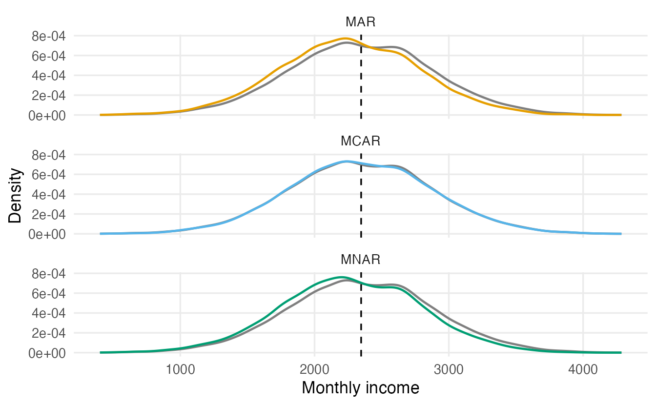
TipHow to read this output
- MCAR: the bias is about -1, essentially zero (the remaining difference is random noise). Losing 30% of the data made the estimate less precise, but not systematically wrong.
- MAR: the respondents are younger, hence poorer, on average. The complete-case mean underestimates the truth by about 87.
- MNAR: high earners hide their income, and the mean is too low by about 78.
Using the observed information
Under MAR the bias comes from age, which we observe. If we use age to predict the missing incomes (here with a simple linear regression fitted on the complete cases), most of the bias disappears. Under MNAR the same trick helps only partly, because the reason for missingness — income itself — is exactly what we do not see:
reg_mean <- sapply(missing, \(m) {
  fit <- lm(income ~ age, subset = !m)          # fit on observed rows
  filled <- income
  filled[m] <- predict(fit, newdata = data.frame(age = age[m]))
  mean(filled)
})
round(rbind(complete_case = cc_mean - true_mean,
            regression_fill = reg_mean - true_mean), 1)
#> MCAR MAR MNAR
#> complete_case -0.6 -87.1 -77.6
#> regression_fill 2.9 -4.2 -44.4This is the key idea behind modern methods such as multiple imputation (Section 9): use everything you observe to make the missing-at-random assumption as plausible as possible. (Filling in single predicted values, as we just did, fixes the mean but still understates uncertainty — more on that next.)
6. Removing missing values
Inside a computation: na.rm = TRUE
Most summary functions have an na.rm argument: mean(), median(), sd(), var(), sum(), min(), max(), quantile(). For correlations, use use = "complete.obs":
mean(airquality$Ozone, na.rm = TRUE)#> [1] 42.13cor(airquality$Ozone, airquality$Temp, use = "complete.obs")#> [1] 0.6984Dropping rows: drop_na() and na.omit()
tidyr::drop_na() removes rows with missing values — in any column, or only in the columns you name. Base R’s na.omit() always looks at all columns.
nrow(titanic)#> [1] 418nrow(na.omit(titanic)) # any column missing -> row dropped#> [1] 87nrow(drop_na(titanic)) # same#> [1] 87nrow(drop_na(titanic, Age)) # only rows with missing Age dropped#> [1] 332Dropping every incomplete row keeps only 87 of 418 passengers, almost entirely because of Cabin, a column we may not even need. Drop rows only for the variables your analysis uses, and report how many rows you lost. Remember from Section 5: complete-case analysis is safe under MCAR but may be biased otherwise.
7. Replacing missing values with a constant: replace_na()
Sometimes a missing value has a known meaning. For the Titanic, a missing Cabin usually means that no cabin number was recorded, so an explicit category is more honest than dropping the passenger:
titanic |>
  mutate(Cabin = replace_na(Cabin, "Unknown")) |>
  count(cabin_known = Cabin != "Unknown")
#> # A tibble: 2 × 2
#> cabin_known n
#> <lgl> <int>
#> 1 FALSE 327
#> 2 TRUE 91For numeric data, replace NA by 0 only when “missing” really means “zero” (e.g. no purchases recorded = 0 purchases). For a measurement such as age or ozone, 0 is a wrong value, not a missing one.
9. Doing it properly: multiple imputation
Multiple imputation (MI) addresses both problems of single imputation:
- it predicts each missing value from the other variables (as in Section 5), which removes bias under MAR;
- it adds random noise to those predictions and repeats the whole process several times (say 5–20), creating several completed datasets. The analysis is run on each, and the results are combined (with “Rubin’s rules”) so that standard errors include the extra uncertainty due to the missing values.
In R the standard package is mice (Multivariate Imputation by Chained Equations). A minimal workflow looks like this:
imp  <- mice::mice(airquality, m = 20, seed = 1, printFlag = FALSE)  # 20 datasets
fits <- with(imp, lm(Ozone ~ Temp + Wind))       # fit the model on each
summary(mice::pool(fits))                        # combine the results
MI is not magic: it relies on the MAR assumption and on a sensible imputation model. But it is the recommended default when missingness is more than trivial. The free online book by van Buuren (below) is the reference.
WarningCommon pitfalls
- Testing
x == NA. AlwaysNA. Useis.na(x). - Forgetting
na.rm = TRUEand gettingNA— or, worse, silently using a function that dropsNAs without telling you how many. na.omit()on the whole data frame, losing most rows because of a column you do not need. Drop on the variables you analyse, and report the loss.- Assuming complete-case analysis is harmless. It is unbiased only if data are MCAR (or, for regression, if missingness depends only on the predictors).
- Mean imputation followed by tests and confidence intervals. The variance is underestimated and the p-values are too small. Use multiple imputation, or at least report the analysis with and without imputation.
- Missing-value codes left as numbers (
-99,999). Convert them toNAat import (see Importing data).
10. Check your understanding
11. Exercises
Interactive (run in your browser)
★ Exercise 1 — how much is missing? For the built-in airquality, compute (a) the proportion of missing values in each column and (b) the proportion of rows that are complete.
is.na(df) gives a logical matrix; colMeans() of it gives proportions. complete.cases(df) gives one TRUE/FALSE per row.
colMeans(is.na(airquality))
mean(complete.cases(airquality))   # about 0.73
About 24% of Ozone and 5% of Solar.R values are missing; roughly 73% of the days are complete.
★★ Exercise 2 — predict the output. Write down what each line returns before running the code.
NA propagates unless the answer is the same whatever the unknown value is. Is NA & FALSE the same whether NA is TRUE or FALSE?
NA, 14, 0.5, 4 10, NA, FALSE. The last one is FALSE because “anything AND FALSE” is FALSE regardless of the unknown value — R only returns NA when the answer really is unknown.
★★ Exercise 3 — the cost of mean imputation. Impute the missing Solar.R values of airquality with the mean, then compare (a) the standard deviation and (b) the correlation with Ozone (using complete cases) before and after imputation.
The replacement value is mean(Solar.R, na.rm = TRUE); the second standard deviation is of aq$solar_imp.
aq <- airquality |>
  mutate(Solar.R   = as.numeric(Solar.R),
         solar_imp = replace_na(Solar.R, mean(Solar.R, na.rm = TRUE)))
c(before = sd(aq$Solar.R, na.rm = TRUE), after = sd(aq$solar_imp))
c(before = cor(aq$Solar.R, aq$Ozone, use = "complete.obs"),
  after  = cor(aq$solar_imp, aq$Ozone, use = "complete.obs"))
Both the standard deviation and the correlation decrease slightly. The effect is small here because only 7 of 153 values (about 5%) were imputed; with 30–50% missing it becomes large.
★★★ Exercise 4 — simulate MCAR vs MNAR. The code creates exam scores for 5,000 students. Make the score missing (a) completely at random with probability 0.4, and (b) with a probability that is higher for low scores (students with low scores do not report them). Compare the mean of the observed scores with the true mean in both cases.
For MCAR the probability is the constant 0.4. For MNAR the probability must depend on score: plogis(6 - 0.3 * score) is larger for small scores.
miss_mcar <- runif(5000) < 0.4
miss_mnar <- runif(5000) < plogis(6 - 0.3 * score)
c(mcar = mean(score[!miss_mcar]) - true_mean,
  mnar = mean(score[!miss_mnar]) - true_mean)
The MCAR difference is close to 0. Under MNAR the observed mean is too high (by roughly 1 point): the students who did not report were mostly the weaker ones. Nothing in the observed scores alone reveals this.
Practice on your own computer
★★ Exercise 5 — group-wise imputation on the Titanic. Read data/test.csv. Impute the missing Age values (a) with the overall median and (b) with the median of each Pclass × Sex group. Compare the mean imputed age of third-class passengers under the two methods, and the standard deviation of Age before and after each imputation.
TipSolution
library(dplyr)
library(tidyr)
library(readr)

titanic <- read_csv(here::here("data", "test.csv"), show_col_types = FALSE)

titanic_imp <- titanic |>
  mutate(age_overall = replace_na(Age, median(Age, na.rm = TRUE))) |>
  mutate(age_group = replace_na(Age, median(Age, na.rm = TRUE)),
         .by = c(Pclass, Sex))

titanic_imp |>
  filter(is.na(Age)) |>
  summarise(overall = mean(age_overall), by_group = mean(age_group),
            .by = Pclass)

titanic_imp |>
  summarise(across(c(Age, age_overall, age_group), \(v) sd(v, na.rm = TRUE)))
First-class passengers are older on average than third-class ones; the group-wise median gives third-class passengers younger imputed ages, which is more plausible. Both imputations reduce the standard deviation compared with the observed Age, the group-wise one less so.
★★★ Exercise 6 — compare three analyses. Using airquality, estimate the slope of Temp in lm(Ozone ~ Temp) with (a) complete cases, (b) mean-imputed Ozone, and (c) multiple imputation with mice (m = 20, seed = 1). Compare the slopes and their standard errors.
TipSolution
library(dplyr)
library(tidyr)

cc  <- lm(Ozone ~ Temp, data = airquality)
aq_mean <- airquality |>
  mutate(Ozone = replace_na(as.numeric(Ozone), mean(Ozone, na.rm = TRUE)))
mean_fit <- lm(Ozone ~ Temp, data = aq_mean)

imp  <- mice::mice(airquality, m = 20, seed = 1, printFlag = FALSE)
mi   <- summary(mice::pool(with(imp, lm(Ozone ~ Temp))))

summary(cc)$coefficients["Temp", 1:2]
summary(mean_fit)$coefficients["Temp", 1:2]
mi[mi$term == "Temp", c("estimate", "std.error")]
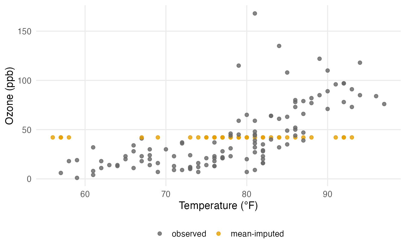
Mean imputation gives a flatter slope (the imputed points lie on a horizontal line) and a smaller standard error (it pretends to have 153 real observations). Complete-case and multiple-imputation slopes are similar here, with MI using the information in the other variables.
Summary
| Task | Code |
|---|---|
| Is it missing? | is.na(x), anyNA(x) |
| Count / proportion per column | colSums(is.na(df)), colMeans(is.na(df)) |
| Complete rows | complete.cases(df) |
| Ignore NAs in a summary | mean(x, na.rm = TRUE), cor(x, y, use = "complete.obs") |
| Drop rows | tidyr::drop_na(df, col), na.omit(df) |
| Replace with a constant | tidyr::replace_na(x, value) |
| Mean / group-mean imputation | mutate(x = replace_na(x, mean(x, na.rm = TRUE)), .by = g) |
| Multiple imputation | mice::mice(), with(), mice::pool() |
- The reason values are missing (MCAR, MAR, MNAR) decides whether simple fixes are safe.
- Complete-case analysis is unbiased only under MCAR; under MAR, use the observed variables; MNAR needs assumptions beyond the data.
- Mean imputation shrinks variances, weakens correlations and makes p-values too small.
- Drop rows only for the variables you use, and report how many were lost.
- For serious analyses with non-trivial missingness, use multiple imputation.