Correspondence analysis

A map of the associations in a contingency table — and how to read it correctly

Learn row and column profiles, masses and inertia, run correspondence analysis with ca::ca(), build a correct symmetric map with principal coordinates, and interpret contributions and quality of representation.

Level 4 · Models & learning ⏱ ~80 min Prerequisites: Proportions and the chi-square test, Principal component analysis

Learning objectives

By the end of this lesson you will be able to:

describe a contingency table through row and column profiles, masses and inertia ($\chi^2 / n$);
explain correspondence analysis (CA) as a “PCA for tables” and run it with ca::ca();
distinguish standard and principal coordinates and draw a correct symmetric map;
use contributions and quality of representation (cos²) to decide what a map can tell you;
interpret a CA map without the usual mistakes.

library(dplyr)
library(ggplot2)
library(ca)

1. Why correspondence analysis?

In Proportions and the chi-square test you learnt to ask “are hair colour and eye colour associated?” The chi-square test answers yes or no. But it does not say which hair colours go with which eye colours, nor how the categories relate to each other.

Correspondence analysis (CA) turns a contingency table into a map: categories with similar profiles are drawn close together, and the main patterns of association become directions on the map. It is to a table of counts what PCA is to a table of measurements.

2. The data and the chi-square test

HairEyeColor cross-classifies 592 students by hair colour, eye colour and sex. We collapse over sex:

hair_eye <- margin.table(HairEyeColor, margin = c(1, 2))
hair_eye

#>        Eye
#> Hair    Brown Blue Hazel Green
#>   Black    68   20    15     5
#>   Brown   119   84    54    29
#>   Red      26   17    14    14
#>   Blond     7   94    10    16

chi <- chisq.test(hair_eye)
chi

#> 
#>  Pearson's Chi-squared test
#> 
#> data:  hair_eye
#> X-squared = 138, df = 9, p-value <2e-16

The test gives $\chi^2 =$ 138.3 with 9 degrees of freedom ($(4-1)(4-1)$): overwhelming evidence of association. The Pearson residuals (observed − expected) / √expected show where the association lies:

round(chi$residuals, 1)

#>        Eye
#> Hair    Brown Blue Hazel Green
#>   Black   4.4 -3.1  -0.5  -2.0
#>   Brown   1.2 -1.9   1.4  -0.3
#>   Red    -0.1 -1.7   0.9   2.3
#>   Blond  -5.9  7.0  -2.2   0.6

Large positive residuals (Blond–Blue, Black–Brown) mark combinations that occur much more often than independence would predict. CA will summarise this whole table of residuals in a picture.

3. Profiles, masses and inertia

CA works with proportions, not counts.

A row profile is a row divided by its total: the distribution of eye colours within one hair colour.
The average row profile (the column margins) is the distribution of eye colours in the whole sample.

round(prop.table(hair_eye, margin = 1), 2)    # row profiles

#>        Eye
#> Hair    Brown Blue Hazel Green
#>   Black  0.63 0.19  0.14  0.05
#>   Brown  0.42 0.29  0.19  0.10
#>   Red    0.37 0.24  0.20  0.20
#>   Blond  0.06 0.74  0.08  0.13

round(prop.table(margin.table(hair_eye, 2)), 2)  # average profile

#> Eye
#> Brown  Blue Hazel Green 
#>  0.37  0.36  0.16  0.11

Blond-haired students have a very different profile from the average (74% blue eyes versus 36% overall), while brown-haired students are close to the average.

The mass of a row is its share of the total ($n_{i+}/n$). Heavy rows (many people) weigh more in the analysis.
The inertia of a table measures how far the profiles are, on average, from the average profile. It equals

\[ \text{total inertia} = \frac{\chi^2}{n}. \]

n <- sum(hair_eye)
unname(chi$statistic / n)

#> [1] 0.2336

If hair and eye colour were independent, every row profile would equal the average profile and the inertia would be 0. CA decomposes this inertia into dimensions, just as PCA decomposes variance into components.

Going deeper: chi-square distances

The distance between a row profile $a_i$ and the average profile $c$ is the chi-square distance

\[ d^2(a_i, c) = \sum_j \frac{(a_{ij} - c_j)^2}{c_j}. \]

Dividing by $c_j$ gives more weight to differences in rare columns. The total inertia is the mass-weighted average of these squared distances: $\sum_i r_i \, d^2(a_i, c) = \chi^2/n$, where $r_i$ is the row mass. The same holds for columns.

4. Running CA

ca_he <- ca(hair_eye)
ca_he

#> 
#>  Principal inertias (eigenvalues):
#>            1        2        3       
#> Value      0.208773 0.022227 0.002598
#> Percentage 89.37%   9.52%    1.11%   
#> 
#> 
#>  Rows:
#>            Black    Brown     Red  Blond
#> Mass     0.18243  0.48311  0.1199 0.2145
#> ChiDist  0.55119  0.15946  0.3548 0.8384
#> Inertia  0.05543  0.01228  0.0151 0.1508
#> Dim. 1  -1.10428 -0.32446 -0.2835 1.8282
#> Dim. 2   1.44092 -0.21911 -2.1440 0.4667
#> 
#> 
#>  Columns:
#>            Brown   Blue    Hazel    Green
#> Mass     0.37162 0.3632  0.15710  0.10811
#> ChiDist  0.50049 0.5537  0.28865  0.38573
#> Inertia  0.09309 0.1113  0.01309  0.01608
#> Dim. 1  -1.07713 1.1981 -0.46529  0.35401
#> Dim. 2   0.59242 0.5564 -1.12278 -2.27412

A 4 × 4 table has at most $\min(4, 4) - 1 = 3$ dimensions. The principal inertias (eigenvalues) are the squared singular values:

eig <- ca_he$sv^2
data.frame(dim = seq_along(eig),
           inertia = round(eig, 4),
           percent = round(100 * eig / sum(eig), 1),
           cumulative = round(100 * cumsum(eig) / sum(eig), 1))

#>   dim inertia percent cumulative
#> 1   1  0.2088    89.4       89.4
#> 2   2  0.0222     9.5       98.9
#> 3   3  0.0026     1.1      100.0

How to read this output

The inertias add up to the total inertia: 0.2336 = $\chi^2/n$.
Dimension 1 alone accounts for 89.4% of the inertia, dimension 2 for 9.5%. Together, a two-dimensional map shows 98.9% of the association in the table — almost all of it.

5. Standard versus principal coordinates

This is the point where most mistakes happen, so let’s be careful. ca() returns standard coordinates in rowcoord and colcoord. Each dimension of standard coordinates has (weighted) variance 1 — they do not reflect how important the dimension is.

Principal coordinates are standard coordinates multiplied by the singular value of each dimension:

\[ \text{principal} = \text{standard} \times \sqrt{\text{inertia of the dimension}}. \]

In principal coordinates, the spread of the points along each axis reflects the inertia of that axis, and the distances between rows (or between columns) approximate their chi-square distances.

row_pc <- sweep(ca_he$rowcoord, 2, ca_he$sv, `*`)   # principal coordinates
col_pc <- sweep(ca_he$colcoord, 2, ca_he$sv, `*`)
round(row_pc[, 1:2], 3)

#>         Dim1   Dim2
#> Black -0.505  0.215
#> Brown -0.148 -0.033
#> Red   -0.130 -0.320
#> Blond  0.835  0.070

round(col_pc[, 1:2], 3)

#>         Dim1   Dim2
#> Brown -0.492  0.088
#> Blue   0.547  0.083
#> Hazel -0.213 -0.167
#> Green  0.162 -0.339

The symmetric map — the standard CA plot — shows both rows and columns in principal coordinates. That is what plot() draws by default:

plot(ca_he, map = "symmetric")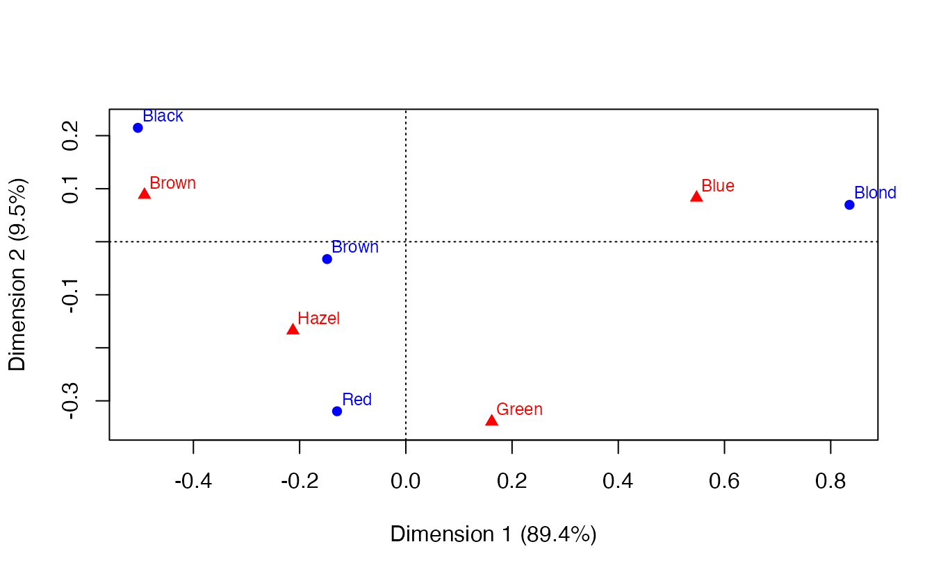

Figure 1: Symmetric CA map of hair colour (blue) and eye colour (red), both in principal coordinates.

The same map with ggplot:

pct <- round(100 * eig / sum(eig), 1)

ca_map <- bind_rows(
  data.frame(label = ca_he$rownames, dim1 = row_pc[, 1], dim2 = row_pc[, 2],
             type = "Hair"),
  data.frame(label = ca_he$colnames, dim1 = col_pc[, 1], dim2 = col_pc[, 2],
             type = "Eye")
)

ggplot(ca_map, aes(dim1, dim2, colour = type, shape = type)) +
  geom_hline(yintercept = 0, colour = "grey70") +
  geom_vline(xintercept = 0, colour = "grey70") +
  geom_point(size = 3) +
  geom_text(aes(label = label), vjust = -0.9, show.legend = FALSE) +
  coord_equal() +
  labs(x = paste0("Dimension 1 (", pct[1], "%)"),
       y = paste0("Dimension 2 (", pct[2], "%)"),
       colour = NULL, shape = NULL)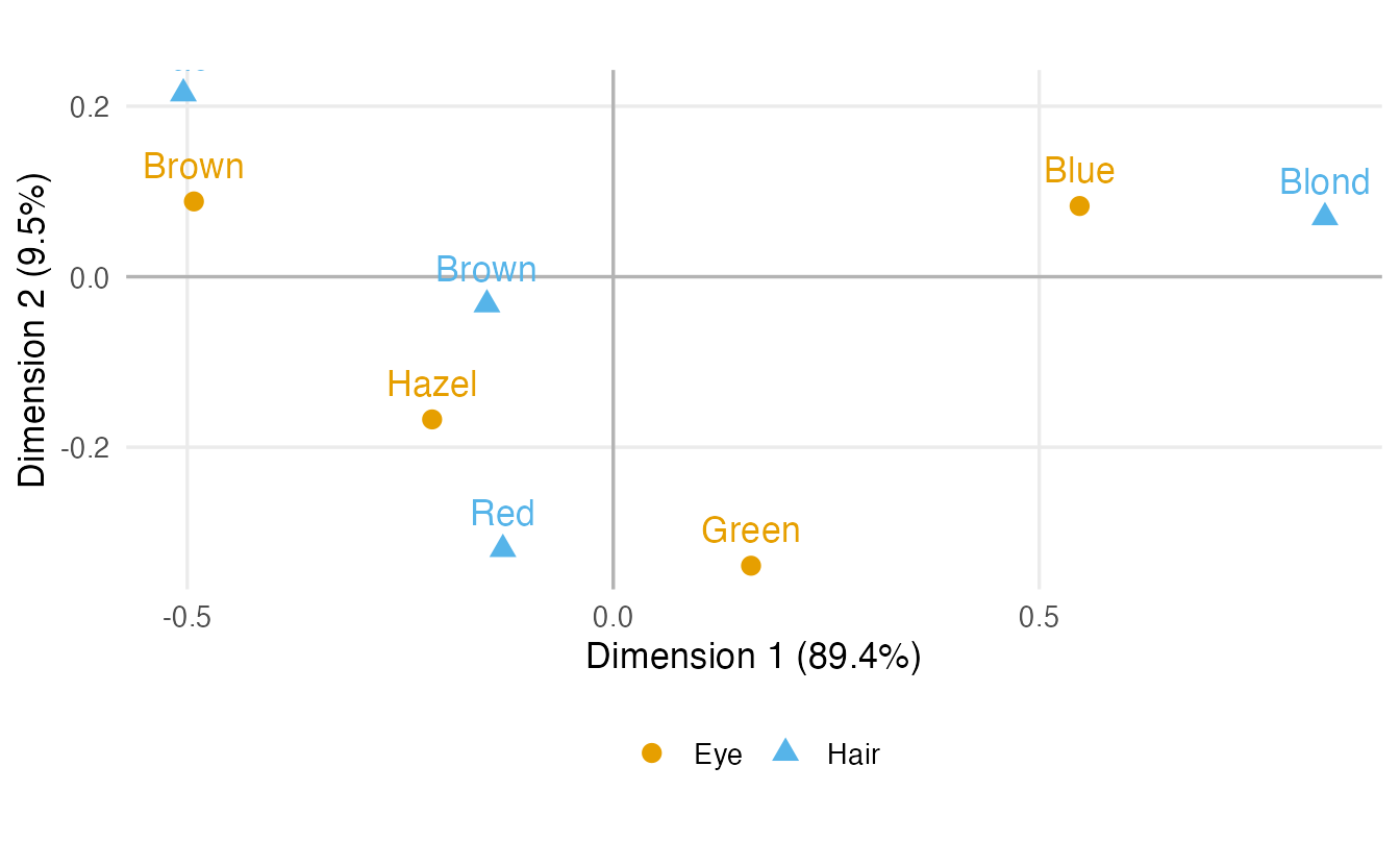

Figure 2: Symmetric CA map built from principal coordinates. Axis labels show the percentage of inertia.

coord_equal() matters: one unit on each axis must have the same length, otherwise distances on the map are distorted.

Going deeper: CA as an SVD of standardised residuals

Let $P = N/n$ be the table of proportions, $r$ and $c$ the row and column masses, and $D_r = \mathrm{diag}(r)$, $D_c = \mathrm{diag}(c)$. CA is the singular value decomposition of the matrix of standardised residuals

\[ S = D_r^{-1/2}\,(P - r c^\top)\,D_c^{-1/2} = U \Sigma V^\top . \]

Each element of $S$ is a Pearson residual divided by $\sqrt n$, so $\sum_{ij} s_{ij}^2 = \chi^2/n$, and the squared singular values $\sigma_k^2$ are the principal inertias. Then

standard coordinates: rows $D_r^{-1/2} U$, columns $D_c^{-1/2} V$;
principal coordinates: rows $D_r^{-1/2} U \Sigma$, columns $D_c^{-1/2} V \Sigma$.

We can verify it by hand:

P  <- hair_eye / n
rm <- rowSums(P)
cm <- colSums(P)
S  <- diag(1 / sqrt(rm)) %*% (P - rm %o% cm) %*% diag(1 / sqrt(cm))
s  <- svd(S)

s$d[1:3]^2                                # principal inertias

#> [1] 0.208773 0.022227 0.002598

ca_he$sv^2                                # same, from ca()

#> [1] 0.208773 0.022227 0.002598

all.equal(abs(diag(1 / sqrt(rm)) %*% s$u[, 1:3]),
          abs(unname(ca_he$rowcoord)))    # standard row coordinates

#> [1] TRUE

(As in PCA, the sign of each dimension is arbitrary, so we compare absolute values.)

6. Reading the map correctly

In a symmetric map, use these rules:

Distances among rows (hair colours) approximate the chi-square distances between their profiles: hair colours close together have similar eye-colour distributions. The same holds among columns.
Distance from the origin: the origin is the average profile. Categories far from the origin have profiles very different from the average; categories near the origin are “average”.
Row–column relationships are read through directions, not distances: a row and a column that lie in the same direction from the origin, both far from it, are positively associated (more frequent together than expected); opposite directions mean they co-occur less than expected.
Distances between a row point and a column point are not directly interpretable in a symmetric map. The two sets of points are on different scales. (The asymmetric maps, plot(ca_he, map = "rowprincipal"), allow a stricter reading of row–column relations, at the cost of a less compact picture.)

What the hair–eye map shows

Dimension 1 (89.4%) is a light–dark axis. Blond hair and blue eyes lie together at one end; black and, less extremely, brown hair lie with brown eyes at the other. This matches the largest residuals: Blond–Blue (7) and Black–Brown (4.4).
Dimension 2 (9.5%) separates red hair and green (and partly hazel) eyes from black hair (residual Red–Green: 2.3).
Brown hair is close to the origin: its eye-colour profile is close to the average, as we saw in the profiles.

Avoid reading quadrants as categories (“quadrant I = …”): the axes’ signs are arbitrary and the quadrants have no meaning in themselves.

7. Contributions and quality of representation

Two diagnostics help you decide which points drive a dimension and which points are faithfully shown.

The contribution of a row to a dimension is the share of that dimension’s inertia due to the row: $\text{mass} \times (\text{standard coordinate})^2$. Contributions to each dimension add up to 1.
The quality of representation of a row on a dimension (cos²) is the share of the row’s own inertia that the dimension shows: $(\text{principal coordinate})^2 / (\text{chi-square distance to the centroid})^2$. Summed over dimensions 1 and 2 it tells you how well the point is represented on the map (1 = perfectly).

row_ctr  <- ca_he$rowmass * ca_he$rowcoord[, 1:2]^2
row_cos2 <- row_pc[, 1:2]^2 / ca_he$rowdist^2
col_ctr  <- ca_he$colmass * ca_he$colcoord[, 1:2]^2
col_cos2 <- col_pc[, 1:2]^2 / ca_he$coldist^2

round(cbind(ctr = row_ctr, cos2 = row_cos2, quality = rowSums(row_cos2)), 3)

#>        Dim1  Dim2  Dim1  Dim2 quality
#> Black 0.222 0.379 0.838 0.152   0.990
#> Brown 0.051 0.023 0.864 0.042   0.906
#> Red   0.010 0.551 0.133 0.812   0.945
#> Blond 0.717 0.047 0.993 0.007   1.000

round(cbind(ctr = col_ctr, cos2 = col_cos2, quality = rowSums(col_cos2)), 3)

#>        Dim1  Dim2  Dim1  Dim2 quality
#> Brown 0.431 0.130 0.967 0.031   0.998
#> Blue  0.521 0.112 0.977 0.022   1.000
#> Hazel 0.034 0.198 0.542 0.336   0.879
#> Green 0.014 0.559 0.176 0.773   0.948

summary() reports the same quantities, multiplied by 1000 (per mille):

summary(ca_he)

#> 
#> Principal inertias (eigenvalues):
#> 
#>  dim    value      %   cum%   scree plot               
#>  1      0.208773  89.4  89.4  **********************   
#>  2      0.022227   9.5  98.9  **                       
#>  3      0.002598   1.1 100.0                           
#>         -------- -----                                 
#>  Total: 0.233598 100.0                                 
#> 
#> 
#> Rows:
#>     name   mass  qlt  inr    k=1 cor ctr    k=2 cor ctr  
#> 1 | Blck |  182  990  237 | -505 838 222 |  215 152 379 |
#> 2 | Brwn |  483  906   53 | -148 864  51 |  -33  42  23 |
#> 3 |  Red |  120  945   65 | -130 133  10 | -320 812 551 |
#> 4 | Blnd |  215 1000  646 |  835 993 717 |   70   7  47 |
#> 
#> Columns:
#>     name   mass  qlt  inr    k=1 cor ctr    k=2 cor ctr  
#> 1 | Brwn |  372  998  398 | -492 967 431 |   88  31 130 |
#> 2 | Blue |  363 1000  477 |  547 977 521 |   83  22 112 |
#> 3 | Hazl |  157  879   56 | -213 542  34 | -167 336 198 |
#> 4 | Gren |  108  948   69 |  162 176  14 | -339 773 559 |

How to read summary()

mass — share of the total; qlt — quality of representation in the dimensions shown (sum of cos²); inr — share of the total inertia due to this point.
For each dimension k: the principal coordinate, cor (cos², quality on that dimension) and ctr (contribution to the dimension).
Dimension 1 is mainly driven by Blond (contribution 717‰) and, among eye colours, by Blue and Brown (521 and 431‰). Dimension 2 is driven by Red hair and Green eyes.
All points are well represented on the 2-D map; the weakest is Hazel (quality 0.88), which still has part of its inertia on dimension 3.

A point with low quality should not be interpreted from its position on the map: it may look close to another point only because the difference between them lies in a dimension that is not shown.

8. Beyond two variables: multiple correspondence analysis

With more than two categorical variables (e.g. hair, eye and sex, or the answers to a whole survey), use multiple correspondence analysis (MCA). MCA needs one row per individual:

he_df <- as.data.frame(HairEyeColor)
people <- he_df[rep(seq_len(nrow(he_df)), he_df$Freq), c("Hair", "Eye", "Sex")]

mca_fit <- FactoMineR::MCA(people, graph = FALSE)
plot(mca_fit, invisible = "ind")    # show only the categories

(Not run here; it requires the FactoMineR package.) The reading rules are the same as for CA, but the percentages of inertia in MCA are known to be pessimistic, so they should not be compared with those of simple CA.

Common pitfalls

Plotting standard coordinates (rowcoord, colcoord) as if they were the map. Multiply by the singular values (principal coordinates), or use plot(ca_obj).
Interpreting the distance between a row point and a column point in a symmetric map. Read row–column associations through directions from the origin.
Interpreting quadrants or the sign of an axis. Signs are arbitrary.
Interpreting badly represented points (low quality / cos²) from their map position.
Calling “contributions” what are in fact coordinates — contributions are mass × standard coordinate², and they add up to 1 per dimension.
Clustering CA coordinates without a reason. CA is descriptive; if you want groups of categories, say why and use the chi-square distances, not an arbitrary algorithm on a handful of points.

9. Check your understanding

Q1. A 5 × 3 table has total inertia 0.10 and n = 500. What was the chi-square statistic, and how many CA dimensions are there?

$\chi^2 = 0.10 \times 500 = 50$. There are $\min(5, 3) - 1 = 2$ dimensions.

Q2. On a symmetric map the point “Red hair” is very close to the point “Hazel eyes”. Can you conclude that red-haired people mostly have hazel eyes?

No. Row-to-column distances are not interpretable in a symmetric map. Look at directions from the origin, at the residuals or at the row profile of red hair (where in fact brown eyes are the most frequent).

Q3. What is the difference between standard and principal coordinates?

Principal coordinates = standard coordinates × singular value. Principal coordinates reflect the importance (inertia) of each dimension and approximate chi-square distances; standard coordinates have unit weighted variance on each dimension.

10. Exercises

★ Exercise 1 — predict, then check. Collapse HairEyeColor to the Hair × Sex table. (a) How many CA dimensions will it have? (b) Compute its total inertia as $\chi^2/n$. (c) What percentage of inertia will dimension 1 explain?

Solution

hair_sex <- margin.table(HairEyeColor, c(1, 3))
unname(chisq.test(hair_sex)$statistic / sum(hair_sex))   # about 0.0135
ca(hair_sex)$sv^2

$\min(4, 2) - 1 = 1$ dimension. (b) About 0.0135 — far smaller than for hair × eye (≈ 0.23): sex and hair colour are only weakly associated. (c) With a single dimension it explains 100% of the inertia.

★★ Exercise 2 — debug the map. This code draws a “CA map” for hair_eye. What is wrong with it, and how do you fix it?

ca_he <- ca(hair_eye)
plot(rbind(ca_he$rowcoord[, 1:2], ca_he$colcoord[, 1:2]), type = "n")
text(ca_he$rowcoord[, 1:2], ca_he$rownames, col = "blue")
text(ca_he$colcoord[, 1:2], ca_he$colnames, col = "red")

Solution

It plots standard coordinates, which give both dimensions the same spread although dimension 1 has about nine times more inertia than dimension 2. The axes are also not on the same scale. Use principal coordinates and an aspect ratio of 1:

rp <- sweep(ca_he$rowcoord[, 1:2], 2, ca_he$sv[1:2], `*`)
cp <- sweep(ca_he$colcoord[, 1:2], 2, ca_he$sv[1:2], `*`)
plot(rbind(rp, cp), type = "n", asp = 1)
text(rp, ca_he$rownames, col = "blue")
text(cp, ca_he$colnames, col = "red")

or simply plot(ca_he).

★★ Exercise 3 — contributions by hand. For the hair–eye CA, verify that (a) the contributions of the four hair colours to dimension 1 add up to 1; (b) the principal inertia of dimension 1 equals the mass-weighted sum of the squared principal coordinates of the rows.

Solution

sum(ca_he$rowmass * ca_he$rowcoord[, 1]^2)              # 1
row_pc <- ca_he$rowcoord[, 1] * ca_he$sv[1]
c(sum(ca_he$rowmass * row_pc^2), ca_he$sv[1]^2)         # equal, about 0.209

Standard coordinates are normalised so that their weighted sum of squares is 1 on every dimension; multiplying by the singular value rescales it to the dimension’s inertia.

★★ Exercise 4 — interpret. In the summary of the hair–eye CA, Hazel has the lowest quality on the 2-D map, with part of its inertia (about 12%) on dimension 3. What does this imply for statements such as “hazel eyes are halfway between brown and green eyes”?

Solution

Part of what distinguishes the hazel profile is not visible in the plane of dimensions 1–2. Its position on the map is still informative (its quality is fairly high, about 0.88), but fine statements about its exact position relative to other points should be made cautiously. Check qlt before interpreting a point, and look at dimension 3 (plot(ca_he, dim = c(1, 3))) if needed.

★★★ Exercise 5 — mini-analysis. The smoke data in the ca package cross-classify 193 employees of a fictitious company by staff group (senior/junior managers and employees, secretaries) and smoking intensity. (a) Run a chi-square test. (b) Run CA and report the percentage of inertia of the first two dimensions. (c) Draw the symmetric map and describe the main pattern. (d) What does the chi-square test result suggest about how much to trust that pattern?

Solution

data(smoke, package = "ca")
chisq.test(smoke)           # warning: some expected counts are small
ca_smoke <- ca(smoke)
round(100 * ca_smoke$sv^2 / sum(ca_smoke$sv^2), 1)
plot(ca_smoke)
summary(ca_smoke)

The test gives $\chi^2 \approx 16.4$ with 12 df, p ≈ 0.17: no significant association, and R warns that some expected counts are small. CA still runs: dimension 1 explains about 88% of the inertia and opposes non-smokers (with senior employees, SE, and secretaries, SC) to smokers (with junior groups, JM and JE). But with so little evidence of association overall, this pattern is a description of this sample that may not replicate. CA is descriptive; it does not replace the test.

Summary

Idea / function	What it does
`margin.table(x, c(1, 2))`	collapse a multi-way table to two variables
`prop.table(tab, 1)`	row profiles
$\chi^2 / n$	total inertia: how far the profiles are from independence
`ca(tab)`	correspondence analysis (`sv`, `rowcoord`, `colcoord`, masses, distances)
`ca_obj$sv^2`	principal inertias (eigenvalues)
standard × `sv`	principal coordinates
`plot(ca_obj)`	symmetric map (both sets in principal coordinates)
`summary(ca_obj)`	mass, quality, inertia, coordinates, cos², contributions (×1000)
`FactoMineR::MCA()`	multiple CA for several categorical variables

CA decomposes the inertia $\chi^2/n$ of a table into a few dimensions.
A correct symmetric map uses principal coordinates for rows and columns, with equal axis scales.
Interpret distances among rows and among columns; read row–column association through directions from the origin.
Use contributions to name the dimensions and quality (cos²) to decide which points can be interpreted.