GRU networks for text classification

Reading movie reviews word by word — and checking against a bag-of-words baseline

Turn text into padded sequences of word ids, learn word embeddings, understand the update and reset gates of a GRU and how they compare with LSTM, and compare GRU, LSTM and a penalised bag-of-words logistic regression on the IMDB reviews.

Level 4 · Models & learning ⏱ ~90 min Prerequisites: LSTM for time series, Penalised regression

NoteLearning objectives

By the end of this lesson you will be able to:

• turn texts into sequences of word ids and pad them to a fixed length;
• explain what an embedding layer learns;
• describe the update and reset gates of a GRU and compare a GRU with an LSTM (gates, memory, number of parameters);
• fit GRU and LSTM classifiers with layer_gru() / layer_lstm() and early stopping;
• compare them honestly with a penalised bag-of-words logistic regression, and choose a classification threshold.

library(dplyr)
library(tidyr)
library(ggplot2)

library(keras3)

ImportantRunning this lesson

The model chunks need keras3 and a backend (see lesson 61); the IMDB reviews are downloaded by keras the first time (about 20 MB). The baseline uses the CRAN packages glmnet and Matrix. The results on this page were computed once and frozen. Without keras, the keras code is shown but not run, and numbers that depend on it read “not computed”. The small base-R examples (padding, gates, parameter counts) run everywhere.

1. Why read text in order?

A film website receives thousands of reviews a day and wants to know which are positive and which are negative. Each review is a piece of text of variable length; the label is 1 (positive) or 0 (negative). This is binary classification, as in lesson 41 — but the “predictors” are words.

The simplest approach ignores word order: count which words appear (a bag of words) and fit a logistic regression. It works surprisingly well. But order sometimes matters: “not good, not bad, actually great” and “great? actually not good” contain almost the same words. A recurrent network reads the words one at a time, like the LSTM read hours of electricity demand in lesson 64. In this lesson we use the Gated Recurrent Unit (GRU), a simpler relative of the LSTM, and we check whether reading in order actually pays off.

2. The data: 50,000 movie reviews

The IMDB dataset (Maas et al., 2011) ships with keras: 25,000 training and 25,000 test reviews, half positive and half negative. The reviews are already tokenised: each word has been replaced by an integer id, with frequent words getting small ids. We keep only the 10,000 most frequent words; rarer words become a special “unknown” id.

max_words <- 10000
imdb <- dataset_imdb(num_words = max_words)
x_train_raw <- imdb$train$x          # a list: one integer vector per review
y_train     <- imdb$train$y          # 0 = negative, 1 = positive
x_test_raw  <- imdb$test$x
y_test      <- imdb$test$y
c(train = length(x_train_raw), test = length(x_test_raw))

#> train  test 
#> 25000 25000

table(y_train)

#> y_train
#>     0     1 
#> 12500 12500

head(x_train_raw[[1]], 12)

#>  [1]    1   14   22   16   43  530  973 1622 1385   65  458 4468

To read a review we need the dictionary. Ids 0, 1 and 2 are reserved (padding, “start of review”, “unknown word”), so the word with dictionary index \(k\) has id \(k + 3\):

word_index <- dataset_imdb_word_index()            # word -> dictionary index

#> Downloading data from https://storage.googleapis.com/tensorflow/tf-keras-datasets/imdb_word_index.json
#> 
      0/1641221 ━━━━━━━━━━━━━━━━━━━━ 0s 0s/step
  49152/1641221 ━━━━━━━━━━━━━━━━━━━━ 3s 2us/step
  81920/1641221 ━━━━━━━━━━━━━━━━━━━━ 3s 2us/step
 245760/1641221 ━━━━━━━━━━━━━━━━━━━━ 1s 1us/step
 811008/1641221 ━━━━━━━━━━━━━━━━━━━━ 0s 0us/step
1641221/1641221 ━━━━━━━━━━━━━━━━━━━━ 0s 0us/step

index_word <- setNames(names(word_index), unlist(word_index) + 3)
decode <- function(ids) {
  words <- index_word[as.character(ids)]
  words[ids == 1] <- "<start>"
  words[ids == 2] <- "<unk>"
  paste(words, collapse = " ")
}
substr(decode(x_train_raw[[1]]), 1, 300)

#> [1] "<start> this film was just brilliant casting location scenery story direction everyone's really suited the part they played and you could just imagine being there robert <unk> is an amazing actor and now the same being director <unk> father came from the same scottish island as myself so i loved the"

Reviews have very different lengths:

len <- lengths(x_train_raw)
summary(len)

#>    Min. 1st Qu.  Median    Mean 3rd Qu.    Max. 
#>      11     130     178     239     291    2494

mean(len > 200)

#> [1] 0.4271

The median review has 178 words, but 43% are longer than 200 words.

3. From texts to a matrix: padding

A network trains on mini-batches, so all sequences in a batch must have the same length \(T\). We pad short reviews with the id 0 and truncate long ones. By default keras pads and truncates at the start (“pre”): it keeps the last \(T\) words and puts the zeros in front. Here is the same logic in base R on three toy “reviews”:

pad_pre <- function(seqs, maxlen) {
  t(vapply(seqs, \(s) {
    s <- tail(s, maxlen)                       # keep the last maxlen ids
    c(rep(0L, maxlen - length(s)), s)          # zeros in front
  }, integer(maxlen)))
}
toy <- list(c(5L, 12L, 7L), c(3L, 9L, 4L, 8L, 2L, 6L), 11L)
pad_pre(toy, maxlen = 4)

#>      [,1] [,2] [,3] [,4]
#> [1,]    0    5   12    7
#> [2,]    4    8    2    6
#> [3,]    0    0    0   11

The second toy review lost its first two ids; the others got leading zeros. Pre-padding suits recurrent networks: the network’s final state, which is used for the prediction, is reached right after the real words rather than after a long run of zeros.

max_len <- 200
x_train_pad <- pad_sequences(x_train_raw, maxlen = max_len)
x_test_pad  <- pad_sequences(x_test_raw,  maxlen = max_len)
dim(x_train_pad)

#> [1] 25000   200

We set aside 15% of the training reviews as a validation set (for early stopping and for tuning the baseline). The test set is used once, at the end.

set.seed(123)
va_idx <- sample(nrow(x_train_pad), size = round(0.15 * nrow(x_train_pad)))
X_tr <- x_train_pad[-va_idx, ];  y_tr <- y_train[-va_idx]
X_va <- x_train_pad[va_idx, ];   y_va <- y_train[va_idx]
c(train = nrow(X_tr), valid = nrow(X_va))

#> train valid 
#> 21250  3750

4. The baseline: a penalised bag-of-words model

Before any network, a model that ignores order. Each review becomes a row of 10,000 columns, one per word, containing \(\log(1 + \text{count})\). Most entries are zero, so we store the matrix in sparse form (only the non-zero values). A lasso logistic regression (lesson 43) then picks the useful words; we choose the penalty \(\lambda\) with the same validation set the networks will use.

bow_matrix <- function(seqs, V = max_words) {
  m <- Matrix::sparseMatrix(i = rep(seq_along(seqs), lengths(seqs)),
                            j = unlist(seqs), x = 1,
                            dims = c(length(seqs), V))   # repeated words summed
  m@x <- log1p(m@x)                                      # dampen counts
  m
}
bow_all  <- bow_matrix(x_train_raw)
bow_tr   <- bow_all[-va_idx, ]
bow_va   <- bow_all[va_idx, ]
bow_test <- bow_matrix(x_test_raw)

We also need a way to score probabilities. The AUC is the probability that a randomly chosen positive review gets a higher score than a randomly chosen negative one; it can be computed from ranks (it is the Mann–Whitney statistic of lesson 36, rescaled):

auc_rank <- function(p, y) {
  r <- rank(p)
  n1 <- sum(y == 1); n0 <- sum(y == 0)
  (sum(r[y == 1]) - n1 * (n1 + 1) / 2) / (n1 * n0)
}
scores <- function(p, y) c(accuracy = mean((p >= 0.5) == y), auc = auc_rank(p, y))

bow_fit <- glmnet::glmnet(bow_tr, y_tr, family = "binomial")    # lasso path
p_va_path <- predict(bow_fit, bow_va, type = "response")       # one column per lambda
val_auc_path <- apply(p_va_path, 2, auc_rank, y = y_va)
best_lambda <- bow_fit$lambda[which.max(val_auc_path)]
p_va_bow <- as.vector(predict(bow_fit, bow_va, s = best_lambda, type = "response"))
scores(p_va_bow, y_va)

#> accuracy      auc 
#>   0.8939   0.9570

TipHow to read this output

glmnet() fits the lasso for a whole sequence of penalties; we keep the one with the highest validation AUC. Accuracy is the share of validation reviews classified correctly at the threshold 0.5, AUC the ranking quality. A validation AUC of 0.957 from a model that does not know word order is the bar the recurrent networks have to clear. Note that the bag of words sees the whole review, while the networks will see only its last 200 words.

A bonus of the linear model: its coefficients are readable.

b <- as.vector(coef(bow_fit, s = best_lambda))[-1]     # drop the intercept
top <- function(idx) unname(index_word[as.character(idx)])
list(positive = top(order(b, decreasing = TRUE)[1:10]),
     negative = top(order(b)[1:10]))

#> $positive
#>  [1] "finely"       "refreshing"   "ladder"       "cerebral"     "7"           
#>  [6] "greene"       "vengeance"    "delightfully" "wonderfully"  "gently"      
#> 
#> $negative
#>  [1] "vacuous"        "waste"          "disappointment" "worst"         
#>  [5] "poorly"         "believer"       "interminable"   "programming"   
#>  [9] "unwatchable"    "stereotyped"

5. Embeddings: words as vectors

A network could receive each word as a “one-hot” vector of 10,000 zeros and a single one, but that is wasteful and says nothing about which words are similar. An embedding layer is a look-up table: a matrix \(E\) with one row of \(d\) numbers for each word id. Word \(w_t\) is replaced by the row \(e_t = E[w_t, ]\). The entries of \(E\) are ordinary weights, learned by backpropagation together with the rest of the network, so words that play a similar role for the task (“excellent”, “superb”) tend to end up with similar vectors. With 10,000 words and \(d = 32\), the embedding has \(10{,}000 \times 32 =\) 320,000 parameters — by far the largest part of our models.

6. The GRU: two gates instead of three

Lesson 64 explained why a plain RNN forgets: the gradient is multiplied at every step by a factor that is usually smaller than 1. The LSTM fixed this with a separate cell state and three gates. The Gated Recurrent Unit (Cho et al., 2014) keeps the idea but simplifies it: there is only the hidden state \(h_t\), and two gates.

Gate	Question it answers	LSTM counterpart
Update gate \(z_t\)	How much of the old state should I keep, and how much should I replace with new content?	Forget and input gates together
Reset gate \(r_t\)	When proposing new content, how much of the old state should I look at?	(no direct counterpart)

The update gate is the key idea. The new state is a weighted average of the old state and a candidate \(\tilde h_t\) built from the current word:

\[ h_t = z_t \odot h_{t-1} + (1 - z_t) \odot \tilde h_t . \]

When \(z_t\) is close to 1 the state is copied forward almost unchanged; when it is close to 0 it is overwritten. Because the gate depends on the input, the network can learn to keep its memory through unimportant words and write only when something informative arrives.

Let us watch this in base R with a single unit and hand-chosen weights. The input is a “+1” event at step 1, nothing for 14 steps, a “−1” event at step 16, then nothing again. The plain RNN uses \(h_t = \tanh(2x_t + 0.5\,h_{t-1})\). The gated unit uses \(z_t = \sigma(4 - 8|x_t|)\), which is about 0.98 when nothing happens and about 0.02 when an event arrives.

x_seq <- c(1, rep(0, 14), -1, rep(0, 14))
plain_rnn <- function(x) {
  h <- numeric(length(x)); prev <- 0
  for (t in seq_along(x)) { prev <- tanh(2 * x[t] + 0.5 * prev); h[t] <- prev }
  h
}
gated_unit <- function(x) {
  h <- numeric(length(x)); prev <- 0
  for (t in seq_along(x)) {
    z <- 1 / (1 + exp(-(4 - 8 * abs(x[t]))))     # update gate
    prev <- z * prev + (1 - z) * tanh(2 * x[t])   # keep or overwrite
    h[t] <- prev
  }
  h
}

gate_df <- data.frame(step = seq_along(x_seq),
                      plain = plain_rnn(x_seq), gated = gated_unit(x_seq)) |>
  pivot_longer(-step, names_to = "unit", values_to = "state")
ggplot(gate_df, aes(step, state, colour = unit)) +
  geom_hline(yintercept = 0, colour = "grey60") +
  geom_line(linewidth = 0.9) +
  geom_point(size = 1.2) +
  labs(x = "time step", y = "hidden state h", colour = NULL)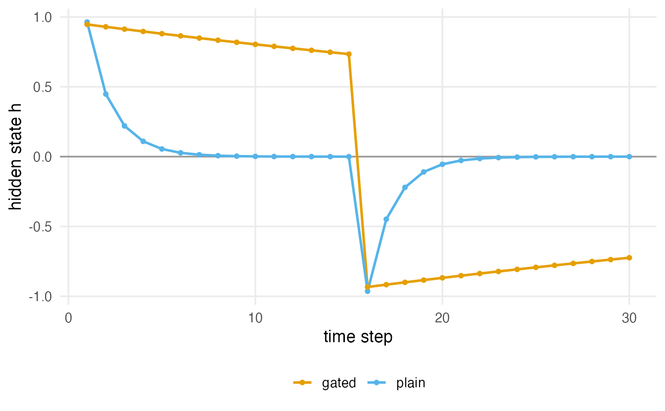

Figure 1: Hidden state of a plain recurrent unit and of a gated (GRU-like) unit after an input event at steps 1 and 16. The plain unit forgets within a few steps; the gated unit keeps the information until a new event overwrites it.

After 14 quiet steps the plain unit’s state is 5.3^{-5} — the first event is forgotten — while the gated unit still holds 0.73. In a real GRU nobody chooses these weights: the gates are small sigmoid layers whose weights are learned from data.

NoteGoing deeper: the GRU equations and its parameter count

With input \(x_t \in \mathbb R^p\) and \(u\) units (this is the convention used by Keras and by Cho et al.; some books swap the roles of \(z_t\) and \(1 - z_t\)):

\[ \begin{aligned} z_t &= \sigma(W_z x_t + U_z h_{t-1} + b_z) && \text{update gate}\\ r_t &= \sigma(W_r x_t + U_r h_{t-1} + b_r) && \text{reset gate}\\ \tilde h_t &= \tanh\big(W_h x_t + r_t \odot (U_h h_{t-1}) + b_h\big) && \text{candidate}\\ h_t &= z_t \odot h_{t-1} + (1 - z_t) \odot \tilde h_t . \end{aligned} \]

There are three blocks of weights (LSTM: four). Keras applies the reset gate after the recurrent multiplication, as written above (reset_after = TRUE), which needs a second bias vector per block, so a GRU layer has \(3\,(u(u+p) + 2u)\) parameters, against \(4\,(u(u+p) + u)\) for an LSTM. Along the direct path, \(\partial h_t / \partial h_{t-1} = z_t\) (element-wise): when the update gate stays near 1, the gradient passes back through many steps — the same trick as the LSTM’s forget gate.

gru_params  <- function(u, p) 3 * (u * (u + p) + 2 * u)
lstm_params <- function(u, p) 4 * (u * (u + p) + u)
c(gru = gru_params(32, 32), lstm = lstm_params(32, 32))

#>  gru lstm 
#> 6336 8320

With 32 units reading 32-dimensional embeddings, the GRU layer has about a quarter fewer parameters than the LSTM layer. GRU versus LSTM in one table:

	LSTM (lesson 64)	GRU
States carried along the sequence	hidden state \(h_t\) and cell state \(c_t\)	hidden state \(h_t\) only
Gates	forget, input, output	update, reset
Weight blocks	4	3
Typical behaviour	slightly more flexible; sometimes better on long, complex sequences	faster per epoch; often similar accuracy

Neither is better in general. In published comparisons they usually perform similarly, and the difference depends on the task; the practical advice is to try both with the same protocol.

7. Building the networks

Both models have the same structure: embedding (32 dimensions) → one recurrent layer of 32 units → a sigmoid output. The dropout argument of the recurrent layer randomly drops parts of its input at each step during training. A small function avoids writing the model twice:

build_text_model <- function(type = c("gru", "lstm"), units = 32) {
  rnn_layer <- switch(match.arg(type), gru = layer_gru, lstm = layer_lstm)
  model <- keras_model_sequential(input_shape = max_len) |>
    layer_embedding(input_dim = max_words, output_dim = 32) |>
    rnn_layer(units = units, dropout = 0.2) |>
    layer_dense(units = 1, activation = "sigmoid")
  model |> compile(optimizer = optimizer_adam(learning_rate = 1e-3),
                   loss = "binary_crossentropy",
                   metrics = list("accuracy", metric_auc(name = "auc")))
  model
}
set_random_seed(123)
gru <- build_text_model("gru")
gru

#> Model: "sequential"
#> ┏━━━━━━━━━━━━━━━━━━━━━━━━━━━━━━━━━━━┳━━━━━━━━━━━━━━━━━━━━━━━━━━┳━━━━━━━━━━━━━━━┓
#> ┃ Layer (type)                      ┃ Output Shape             ┃       Param # ┃
#> ┡━━━━━━━━━━━━━━━━━━━━━━━━━━━━━━━━━━━╇━━━━━━━━━━━━━━━━━━━━━━━━━━╇━━━━━━━━━━━━━━━┩
#> │ embedding (Embedding)             │ (None, 200, 32)          │       320,000 │
#> ├───────────────────────────────────┼──────────────────────────┼───────────────┤
#> │ gru (GRU)                         │ (None, 32)               │         6,336 │
#> ├───────────────────────────────────┼──────────────────────────┼───────────────┤
#> │ dense (Dense)                     │ (None, 1)                │            33 │
#> └───────────────────────────────────┴──────────────────────────┴───────────────┘
#>  Total params: 326,369 (1.24 MB)
#>  Trainable params: 326,369 (1.24 MB)
#>  Non-trainable params: 0 (0.00 B)

TipHow to read this output

• The embedding layer turns each review, a vector of 200 ids, into a \(200 \times 32\) matrix: Output Shape (None, 200, 32). Its 320,000 parameters are the word vectors.
• The GRU reads the 200 steps and returns only its final hidden state, (None, 32), with 6336 parameters (Section 6).
• The dense layer maps those 32 numbers to \(P(\text{positive})\): \(32 + 1 = 33\) parameters.

8. Training with early stopping

As in lessons 62 and 64, early stopping watches the validation loss and restores the best weights. We also record the training time, since speed is one of the arguments for a GRU.

train_text_model <- function(model, epochs = 15) {
  early_stop <- callback_early_stopping(monitor = "val_loss", patience = 2,
                                        restore_best_weights = TRUE)
  seconds <- system.time(
    history <- model |> fit(
      x = X_tr, y = y_tr,
      validation_data = list(X_va, y_va),
      epochs = epochs, batch_size = 128,
      callbacks = list(early_stop), verbose = 0
    )
  )[["elapsed"]]
  list(history = history, seconds = seconds)
}
gru_run <- train_text_model(gru)

as.data.frame(gru_run$history) |>
  filter(!is.na(value), metric %in% c("loss", "auc")) |>
  ggplot(aes(epoch, value, colour = data)) +
  geom_line(linewidth = 0.8) +
  facet_wrap(~ metric, scales = "free_y") +
  labs(x = "Epoch", y = NULL, colour = NULL)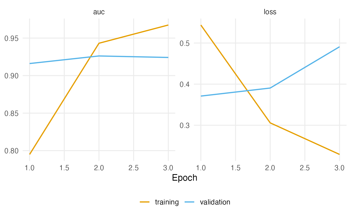

Figure 2: Learning curves of the GRU: loss and AUC on training and validation reviews.

Text models overfit quickly: the training loss keeps falling while the validation loss typically reaches its minimum after only a few epochs. Training stopped after 3 epochs (18 seconds on the instructor’s laptop CPU).

Now the LSTM, with the same seed, data, settings and early stopping:

set_random_seed(123)
lstm <- build_text_model("lstm")
lstm_run <- train_text_model(lstm)

9. The comparison on the test set

Only now do we use the 25,000 test reviews.

p_test <- list(
  bag_of_words = as.vector(predict(bow_fit, bow_test, s = best_lambda,
                                   type = "response")),
  gru  = as.vector(predict(gru,  x_test_pad, verbose = 0)),
  lstm = as.vector(predict(lstm, x_test_pad, verbose = 0))
)
results <- tibble::tibble(
  model   = names(p_test),
  params  = c(sum(b != 0), gru$count_params(), lstm$count_params()),
  seconds = c(NA, gru_run$seconds, lstm_run$seconds),
  accuracy = sapply(p_test, \(p) scores(p, y_test)[["accuracy"]]),
  auc      = sapply(p_test, auc_rank, y = y_test)
)
results

#> # A tibble: 3 × 5
#>   model        params seconds accuracy    auc
#>   <chr>         <int>   <dbl>    <dbl>  <dbl>
#> 1 bag_of_words   2204   NA      0.8845 0.9504
#> 2 gru          326369   18.12   0.8423 0.9190
#> 3 lstm         328353   22.40   0.8614 0.9417

TipHow to read this output

• params is the number of non-zero word coefficients for the lasso and the number of weights for the networks. seconds is the training time (the lasso path is not timed; it takes well under a minute).
• Test AUC: bag of words 0.95, GRU 0.919, LSTM 0.942. With 25,000 test reviews, differences in the second decimal are real; differences in the third decimal are within run-to-run variation (lesson 61, Section 8).
• The usual finding on these data is that GRU and LSTM perform very similarly, and that the bag-of-words lasso is close to both. Reading in order helps with phrases like “not good”, but much of the sentiment is carried by individual words. The network also sees only the last 200 words of each review.

10. From probabilities to decisions

A probability becomes a label only when we choose a threshold. At 0.5, the GRU’s confusion matrix and the usual summaries are:

pred <- as.integer(p_test$gru >= 0.5)
cm <- table(truth = factor(y_test, levels = 0:1), pred = factor(pred, levels = 0:1))
cm

#>      pred
#> truth     0     1
#>     0 10557  1943
#>     1  2000 10500

tp <- cm["1", "1"]; tn <- cm["0", "0"]; fp <- cm["0", "1"]; fn <- cm["1", "0"]
precision <- tp / (tp + fp)
recall    <- tp / (tp + fn)
c(accuracy = (tp + tn) / sum(cm), precision = precision, recall = recall,
  f1 = 2 * precision * recall / (precision + recall))

#>  accuracy precision    recall        f1 
#>    0.8423    0.8438    0.8400    0.8419

Precision answers “of the reviews flagged positive, how many are?”; recall “of the positive reviews, how many did we flag?”; F1 is their harmonic mean. If a marketing team wants to quote only reviews that are surely positive, raise the threshold (higher precision, lower recall); choose it on the validation set, never on the test set.

WarningCommon pitfalls

1. Skipping the bag-of-words baseline. A penalised linear model on word counts is fast, interpretable and often nearly as good as a recurrent network.
2. Forgetting what padding and truncation do. With maxlen = 200 the model never sees the beginning of long reviews; with post-padding, an RNN’s final state is reached after a long run of zeros.
3. Choosing the penalty, the threshold or the number of epochs on the test set. All tuning uses the validation set.
4. Expecting the GRU to beat the LSTM (or vice versa). They usually perform similarly; compare them with the same data, seed and early stopping.
5. Using set.seed() to make keras reproducible. Use set_random_seed(); set.seed() only controls R’s own random numbers (here, the validation split).
6. Ignoring the reserved ids. 0 = padding, 1 = start, 2 = unknown word; the vocabulary size passed to layer_embedding() must be at least the largest id + 1.

11. Check your understanding

NoteQ1. What does an update gate value close to 1 mean in a GRU?

Keep the previous hidden state almost unchanged and ignore the new candidate: the unit “remembers” through this step.

NoteQ2. How many parameters does layer_gru(units = 16) have when it reads 8-dimensional embeddings? And an LSTM of the same size?

GRU: \(3\,(16 \cdot (16 + 8) + 2 \cdot 16) = 3 \cdot 416 = 1248\). LSTM: \(4\,(16 \cdot 24 + 16) = 4 \cdot 400 = 1600\).

NoteQ3. A review has 350 words and maxlen = 200 with the default settings. Which words does the network see?

The last 200: pad_sequences() truncates at the start (truncating = "pre") by default.

NoteQ4. Why is an embedding layer better than one-hot inputs?

It replaces 10,000-dimensional sparse vectors by short dense vectors that are learned for the task, so words with a similar role can get similar representations, and the following layers need far fewer weights.

12. Exercises

★ Exercise 1 — predict the output. Without running it, write down pad_pre(list(c(4L, 8L), c(1L, 2L, 3L, 5L, 7L)), maxlen = 3). What would keras return with padding = "post" and truncating = "post"?

TipSolution

Default (“pre”): rows 0 4 8 and 3 5 7. With padding = "post", truncating = "post": rows 4 8 0 and 1 2 3 — zeros at the end, and the first three ids kept.

★ Exercise 2 — count the parameters. The original version of this lesson used a 128-dimensional embedding followed by layer_bidirectional(layer_gru(units = 64)), which runs one GRU left-to-right and one right-to-left and concatenates their final states. How many parameters does the bidirectional layer have, and what is its output size?

TipSolution

One GRU: \(3\,(64 \cdot (64 + 128) + 2 \cdot 64) = 3 \cdot 12{,}416 = 37{,}248\). Two directions: \(74{,}496\). The output concatenates two 64-vectors: shape (None, 128). You can check with gru_params(64, 128) * 2.

★★ Exercise 3 — a bidirectional GRU. Fit the original lesson’s architecture (embedding 128, bidirectional GRU 64, dense 64 ReLU, dropout 0.3, sigmoid output) with the same split and early stopping, and add it to results. Is the extra size worth it?

TipSolution

set_random_seed(123)
bigru <- keras_model_sequential(input_shape = max_len) |>
  layer_embedding(input_dim = max_words, output_dim = 128) |>
  layer_bidirectional(layer_gru(units = 64, dropout = 0.2)) |>
  layer_dense(units = 64, activation = "relu") |>
  layer_dropout(rate = 0.3) |>
  layer_dense(units = 1, activation = "sigmoid")
bigru |> compile(optimizer = optimizer_adam(1e-3), loss = "binary_crossentropy",
                 metrics = list(metric_auc(name = "auc")))
bigru_run <- train_text_model(bigru)
p_bigru <- as.vector(predict(bigru, x_test_pad, verbose = 0))
scores(p_bigru, y_test)

The model has about 1.36 million parameters (mostly the embedding) and takes several times longer per epoch. Its test AUC is typically within about a hundredth of the small GRU: on this task the extra capacity buys little.

★★ Exercise 4 — GRU for electricity demand. In lesson 64, replace layer_lstm(units = 32) with layer_gru(units = 32) and keep everything else (windows, split, callbacks). Compare test RMSE, number of parameters and training time with the LSTM and with the AR(48) baseline.

TipSolution

set_random_seed(123)
gru_ts <- keras_model_sequential(input_shape = c(L, 1)) |>
  layer_gru(units = 32) |>
  layer_dense(units = 1)
gru_ts |> compile(optimizer = optimizer_adam(1e-3), loss = "mse")
secs <- system.time(
  gru_ts |> fit(w_train$X, w_train$y,
                validation_data = list(w_valid$X, w_valid$y),
                epochs = 30, batch_size = 128, callbacks = callbacks, verbose = 0)
)[["elapsed"]]
forecasts$gru <- to_mwh(as.vector(predict(gru_ts, w_test$X, verbose = 0)))
score(forecasts)
c(params = gru_ts$count_params(), seconds = secs)

The GRU layer has \(3\,(32 \cdot 33 + 64) = 3360\) parameters against 4352 for the LSTM. Its test RMSE is usually very close to the LSTM’s, and both should be compared with AR(48), which uses the same inputs.

★★ Exercise 5 — interpret the errors. Find the 5 test reviews where the GRU is most confidently wrong (largest \(|y - \hat p|\)) and read them with decode(). What do they have in common?

TipSolution

wrong <- order(abs(y_test - p_test$gru), decreasing = TRUE)[1:5]
data.frame(truth = y_test[wrong], p_gru = round(p_test$gru[wrong], 3))
for (i in wrong) cat(substr(decode(x_test_raw[[i]]), 1, 400), "\n\n")

Typical cases: sarcasm, reviews that describe a bad plot before praising the film (or the reverse), long reviews whose opinion is in the part cut off by truncation, and labels that seem debatable. Errors like these are a reminder that the model learns word patterns, not opinions.

★★★ Exercise 6 — is reading in order worth it? Compute a 95% paired bootstrap interval for the difference in test AUC between the GRU and the bag-of-words lasso (resample the same test reviews for both, 500 replicates). Then write two sentences for a non-technical manager recommending one model.

TipSolution

set.seed(1)
d <- replicate(500, {
  i <- sample(length(y_test), replace = TRUE)
  auc_rank(p_test$gru[i], y_test[i]) - auc_rank(p_test$bag_of_words[i], y_test[i])
})
quantile(d, c(0.025, 0.975))

With 25,000 test reviews the interval is narrow, so even a small difference can be “significant”. The recommendation should weigh its size against cost: if the GRU gains only about a hundredth of AUC, the lasso — which trains in seconds, runs anywhere and shows which words drive the prediction — is a defensible choice.

Summary

Idea / code	Meaning
dataset_imdb(num_words = )	Tokenised movie reviews (integer ids)
pad_sequences(x, maxlen = )	Pad / truncate to a fixed length (default: at the start)
layer_embedding(input_dim, output_dim)	Learned look-up table of word vectors
Update gate \(z_t\), reset gate \(r_t\)	Keep-or-overwrite, and how much past to use for the candidate
layer_gru(units = , dropout = )	GRU layer; \(3(u(u+p) + 2u)\) parameters
layer_lstm(), layer_bidirectional()	LSTM; read the sequence in both directions
glmnet::glmnet() on a sparse bag of words	The baseline to beat
Precision, recall, F1, threshold	Turning probabilities into decisions

• A GRU is a simplified LSTM: one state, two gates, three weight blocks; in practice the two perform similarly.
• Texts become padded sequences of ids, then dense vectors through an embedding.
• A penalised bag-of-words model is fast, interpretable and often close to the recurrent networks; always report it.
• All tuning (penalty, epochs, threshold) uses the validation set; the test set is used once.

NoteFurther reading

• keras3, “Working with RNNs” guide, https://keras3.posit.co/articles/working_with_rnns.html
• James et al., An Introduction to Statistical Learning (2e), section 10.5 “Recurrent neural networks” (document classification on IMDB), https://www.statlearning.com
• Silge & Robinson, Text Mining with R, https://www.tidytextmining.com
• Chollet, Kalinowski & Allaire, Deep Learning with R (2nd ed.), Manning, 2022, chapter 11 (text).