t-tests: comparing means

One-sample, two-sample (Welch) and paired t-tests — and how to read them

Learn when and how to use the three t-tests, check their assumptions, report effect sizes and interpret the output without the usual misconceptions.

Level 3 · Inference ⏱ ~75 min Prerequisites: Confidence intervals, Hypothesis testing

NoteLearning objectives

By the end of this lesson you will be able to:

• choose between a one-sample, two-sample and paired t-test;
• run each test with t.test() and read every line of its output;
• check the assumptions that matter (and know which ones matter less);
• report an effect size and a confidence interval, not just a p-value.

library(dplyr)
library(ggplot2)

1. Why do we need a test?

Gentoo penguins look heavier than Adelie penguins. But we only measured a few hundred birds. If we went back to Antarctica and caught a different sample, the two averages would change. The question a t-test answers is:

Is the difference we see between the sample means larger than what random sampling alone would typically produce?

The t-test compares a signal (the difference between means) with the noise we expect from sampling variability (the standard error). If the signal is many times larger than the noise, chance alone is an unlikely explanation.

\[ t \;=\; \frac{\text{signal}}{\text{noise}} \;=\; \frac{\text{observed difference} - \text{difference under } H_0}{\text{standard error of the difference}} \]

2. The three t-tests at a glance

Question	Test	R code
Is the mean of one group different from a reference value?	One-sample	t.test(x, mu = m0)
Do two independent groups have different means?	Two-sample (Welch)	t.test(y ~ group, data = df)
Do two measurements on the same units differ on average?	Paired	t.test(after, before, paired = TRUE)

The key question is about the design, not the data: are the two sets of numbers measured on the same units (paired) or on different units (independent)?

3. One-sample t-test

Suppose a field guide claims that Adelie penguins have a mean flipper length of 190 mm. Do our data agree?

adelie <- penguins |>
  filter(species == "Adelie") |>
  pull(flipper_len)

mean(adelie, na.rm = TRUE)

#> [1] 190

res_one <- t.test(adelie, mu = 190)
res_one

#> 
#>  One Sample t-test
#> 
#> data:  adelie
#> t = -0.087, df = 150, p-value = 0.9
#> alternative hypothesis: true mean is not equal to 190
#> 95 percent confidence interval:
#>  188.9 191.0
#> sample estimates:
#> mean of x 
#>       190

TipHow to read this output

• t — the signal-to-noise ratio: the sample mean is -0.09 standard errors away from 190.
• df — degrees of freedom (\(n - 1\)); they set the exact shape of the t distribution used.
• p-value — if the true mean were 190, a sample mean at least this far from 190 would occur with probability 0.93.
• 95 percent confidence interval — the range of population means that are compatible with the data: from 188.9 to 191 mm. Note that 190 lies inside it — this always agrees with the test at the 5% level.
• sample estimates — the sample mean.

NoteGoing deeper: the one-sample t statistic

With sample mean \(\bar x\), sample standard deviation \(s\) and sample size \(n\),

\[ t = \frac{\bar x - \mu_0}{s / \sqrt{n}}, \qquad t \sim t_{n-1} \text{ under } H_0: \mu = \mu_0 . \]

The denominator \(s/\sqrt n\) is the standard error of the mean (see Sampling distributions). The t distribution has heavier tails than the normal because \(s\) is itself estimated; as \(n\) grows, \(t_{n-1}\) approaches \(N(0,1)\).

4. Two-sample t-test (Welch)

Now the original question: do Adelie and Gentoo penguins differ in body mass? These are different birds, so the samples are independent.

Look first

two_sp <- penguins |>
  filter(species %in% c("Adelie", "Gentoo")) |>
  droplevels()

ggplot(two_sp, aes(species, body_mass, colour = species)) +
  geom_boxplot(outlier.shape = NA, width = 0.5) +
  geom_jitter(width = 0.15, alpha = 0.4) +
  labs(x = NULL, y = "Body mass (g)") +
  theme(legend.position = "none")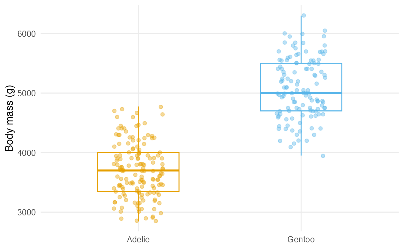

Figure 1: Body mass of Adelie and Gentoo penguins. Each dot is one bird; the boxes summarise the distributions.

Test

res_welch <- t.test(body_mass ~ species, data = two_sp)
res_welch

#> 
#>  Welch Two Sample t-test
#> 
#> data:  body_mass by species
#> t = -23, df = 250, p-value <2e-16
#> alternative hypothesis: true difference in means between group Adelie and group Gentoo is not equal to 0
#> 95 percent confidence interval:
#>  -1491 -1260
#> sample estimates:
#> mean in group Adelie mean in group Gentoo 
#>                 3701                 5076

R runs Welch’s t-test by default. It does not assume that the two groups have the same variance, and it loses almost nothing when variances happen to be equal. This is why modern practice recommends Welch as the default; the classical “Student” version (var.equal = TRUE) is rarely needed.

TipHow to read this output

• The estimated difference (Adelie − Gentoo) is -1375 g.
• The 95% CI for the difference goes from -1491 to -1260 g: Gentoo penguins are, on average, between roughly 1300 and 1500 g heavier.
• df is not an integer: Welch’s correction adjusts the degrees of freedom for unequal variances.
• The p-value is tiny: a difference this large would be extremely surprising if the two species had the same mean mass.

How big is the difference? Effect size

A p-value tells you whether a difference is detectable, not whether it is large. With huge samples, trivial differences become “significant”. Always report an effect size. Cohen’s \(d\) expresses the difference in units of standard deviation:

cohens_d <- function(x, g) {
  g <- droplevels(as.factor(g))
  m  <- tapply(x, g, mean, na.rm = TRUE)
  s  <- tapply(x, g, sd,   na.rm = TRUE)
  n  <- tapply(!is.na(x), g, sum)
  s_pooled <- sqrt(((n[1] - 1) * s[1]^2 + (n[2] - 1) * s[2]^2) / (sum(n) - 2))
  unname((m[2] - m[1]) / s_pooled)
}

d <- cohens_d(two_sp$body_mass, two_sp$species)
d

#> [1] 2.868

A common (rough!) guide reads \(|d| \approx 0.2\) as small, \(0.5\) as medium and \(0.8\) as large. Here \(d =\) 2.9: an enormous difference — the two distributions barely overlap, as the plot already showed.

NoteGoing deeper: Welch’s statistic

\[ t = \frac{\bar x_1 - \bar x_2}{\sqrt{\dfrac{s_1^2}{n_1} + \dfrac{s_2^2}{n_2}}} \]

The reference distribution is approximately \(t_\nu\) with Welch–Satterthwaite degrees of freedom

\[ \nu \approx \frac{\left(s_1^2/n_1 + s_2^2/n_2\right)^2}{\dfrac{(s_1^2/n_1)^2}{n_1-1} + \dfrac{(s_2^2/n_2)^2}{n_2-1}} . \]

Student’s version replaces the denominator with a pooled variance and uses \(n_1+n_2-2\) degrees of freedom; it is exact only when the population variances are equal.

5. Paired t-test

The built-in sleep data record the extra hours of sleep for the same 10 patients under two drugs. Each patient is their own control, so the measurements are paired.

sleep_wide <- data.frame(
  drug1 = sleep$extra[sleep$group == 1],
  drug2 = sleep$extra[sleep$group == 2]
)
sleep_wide$diff <- sleep_wide$drug2 - sleep_wide$drug1
sleep_wide

#>    drug1 drug2 diff
#> 1    0.7   1.9  1.2
#> 2   -1.6   0.8  2.4
#> 3   -0.2   1.1  1.3
#> 4   -1.2   0.1  1.3
#> 5   -0.1  -0.1  0.0
#> 6    3.4   4.4  1.0
#> 7    3.7   5.5  1.8
#> 8    0.8   1.6  0.8
#> 9    0.0   4.6  4.6
#> 10   2.0   3.4  1.4

res_paired <- t.test(sleep_wide$drug2, sleep_wide$drug1, paired = TRUE)
res_paired

#> 
#>  Paired t-test
#> 
#> data:  sleep_wide$drug2 and sleep_wide$drug1
#> t = 4.1, df = 9, p-value = 0.003
#> alternative hypothesis: true mean difference is not equal to 0
#> 95 percent confidence interval:
#>  0.7001 2.4599
#> sample estimates:
#> mean difference 
#>            1.58

A paired test is simply a one-sample t-test on the differences:

t.test(sleep_wide$diff, mu = 0)$p.value

#> [1] 0.002833

res_paired$p.value

#> [1] 0.002833

What if we (wrongly) ignore the pairing?

t.test(sleep_wide$drug2, sleep_wide$drug1)$p.value

#> [1] 0.07939

Ignoring the pairing throws away information: the patient-to-patient variability is mixed into the noise, the standard error grows and the p-value becomes 0.079 instead of 0.0028. The design determines the test.

6. Assumptions: what really matters

Assumption	How much does it matter?	How to check
Independence of observations (within and, for Welch, between groups)	Crucial. No test fixes a flawed design.	Think about how data were collected.
Approximately normal data (or differences, for paired)	Matters for small \(n\) (say < 30 per group) and strong skew/outliers. For larger \(n\) the Central Limit Theorem helps.	Histogram / QQ-plot; look for strong skew or outliers.
Equal variances	Not needed with Welch (the default).	—

ggplot(two_sp, aes(sample = body_mass)) +
  stat_qq(alpha = 0.5) +
  stat_qq_line(colour = "#E8613C") +
  facet_wrap(~ species) +
  labs(x = "Theoretical quantiles", y = "Sample quantiles")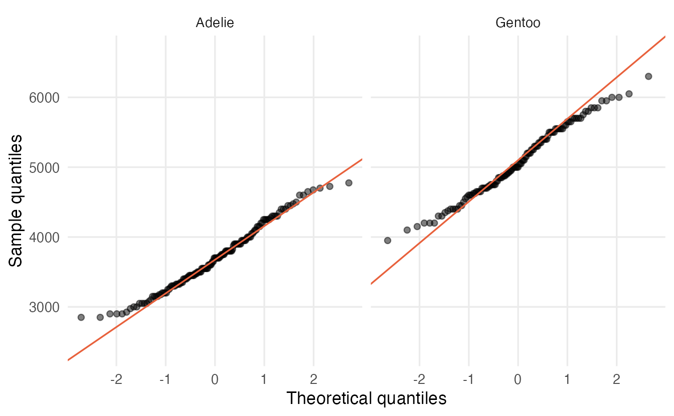

Figure 2: QQ-plots of body mass by species: points close to the line indicate approximate normality.

If samples are small and clearly non-normal, use a rank-based alternative such as the Wilcoxon test (see Non-parametric tests) or a permutation test.

WarningCommon pitfalls

1. “p = 0.03 means there is a 3% chance that H0 is true.” No. The p-value is computed assuming H0 is true; it is a statement about the data, not about the hypothesis.
2. “Not significant” ≠ “no difference”. A large p-value may simply reflect a small sample. Look at the confidence interval: is it narrow around zero, or wide?
3. Using an unpaired test on paired data (or vice-versa). Decide from the design.
4. Running many t-tests on many groups. With 5 groups there are 10 pairwise tests and the chance of at least one false positive grows quickly — use ANOVA and adjusted comparisons.
5. Testing normality with a formal test and then choosing the test. With small samples such tests have little power; with large samples they flag irrelevant deviations. Look at the plots.

7. Check your understanding

NoteQ1. A researcher measures blood pressure on 20 patients before and after a treatment. Which test?

A paired t-test (paired = TRUE): the same patients are measured twice.

NoteQ2. True or false: a 95% CI for a difference that does not contain 0 corresponds to p < 0.05 for the two-sided test.

True (for the same test and the same data). CI and test are two views of the same calculation.

NoteQ3. Why does R use Welch’s version by default?

Because it remains valid when the two variances differ, and it is almost as powerful as Student’s test when they are equal. There is little to lose and a lot to gain.

8. Exercises

Interactive (run in your browser)

★ Exercise 1 — one-sample test. Test whether the mean mpg of the cars in mtcars differs from 20 miles per gallon. Store the result in res and print it.

Use the mpg column with mtcars$mpg, and the reference value 20.

res <- t.test(mtcars$mpg, mu = 20)
res

The p-value is large and the 95% CI contains 20: the data are compatible with a mean of 20 mpg.

★★ Exercise 2 — two independent groups. Do cars with manual transmission (am == 1) have a different mean mpg from automatic cars (am == 0)? Use the formula interface.

The formula is outcome ~ group.

t.test(mpg ~ am, data = mtcars)

Manual cars have a higher mean mpg; the CI for the difference (automatic − manual) lies entirely below 0.

★★★ Exercise 3 — what does “5%” mean? Simulate 5,000 experiments in which there is no true difference: each time draw two samples of size 10 from the same normal distribution and record the Welch p-value. What proportion of p-values is below 0.05? Then repeat with a true difference of 0.8 standard deviations in the second group — what are you estimating now?

Under H0 you should get close to 0.05 — that is the definition of the type I error rate. For the second part, set mean = 0.8.

p_alt <- replicate(5000, {
  x <- rnorm(10); y <- rnorm(10, mean = 0.8)
  t.test(x, y)$p.value
})
mean(p_alt < 0.05)   # about 0.39

The first proportion estimates the type I error rate (≈ 0.05). The second estimates the power of the test for a large effect with only 10 units per group — well below the conventional 80%. Small studies frequently miss real effects.

Practice on your own computer

★★ Exercise 4. Using penguins, compare the bill length (bill_len) of male and female Chinstrap penguins. (a) Plot the data. (b) Run the appropriate test. (c) Report the result in one sentence that includes the estimated difference, its 95% CI and Cohen’s \(d\).

TipSolution

chin <- penguins |>
  filter(species == "Chinstrap", !is.na(sex)) |>
  droplevels()

ggplot(chin, aes(sex, bill_len)) + geom_boxplot() + geom_jitter(width = .1)

res <- t.test(bill_len ~ sex, data = chin)
res
cohens_d(chin$bill_len, chin$sex)

Example report: “Male Chinstrap penguins had longer bills than females (difference ≈ 4.5 mm, 95% CI from about 3.3 to 5.7 mm; Welch t-test, p < 0.001), a very large effect (d ≈ 1.8).” — check the exact numbers in your own output.

★★ Exercise 5 — interpret, don’t compute. A study reports: “t(48) = 1.20, p = 0.24, 95% CI for the difference [−1.1, 4.3]”. A colleague concludes that “the treatment has no effect”. Write two sentences explaining why this conclusion is too strong.

TipSolution

The test did not detect a difference, but the CI shows that the data are compatible with anything from a small negative effect (−1.1) to a fairly large positive effect (4.3). The study is inconclusive — probably under-powered — rather than evidence of no effect.

Summary

Situation	Code	Report
One mean vs reference	t.test(x, mu = m0)	mean, 95% CI, p
Two independent groups	t.test(y ~ g, data = df) (Welch)	difference, 95% CI, p, Cohen’s d
Paired measurements	t.test(x2, x1, paired = TRUE)	mean difference, 95% CI, p

• The t statistic is signal / noise.
• Choose the test from the design (paired vs independent), not from the data.
• Welch is the sensible default for two groups.
• Always report an effect size and a confidence interval alongside the p-value.

NoteFurther reading

• Wickham, Çetinkaya-Rundel & Grolemund, R for Data Science (2e), https://r4ds.hadley.nz
• Çetinkaya-Rundel & Hardin, Introduction to Modern Statistics (2e), chapters on inference for means, https://openintro-ims.netlify.app
• Lakens, D., Improving Your Statistical Inferences, https://lakens.github.io/statistical_inferences/