Spectral clustering

Cluster by connectivity, not by distance to a centre — build it yourself, then use kernlab

Similarity graphs, the graph Laplacian and its eigenvectors; a complete spectral clustering in a few lines of base R that separates concentric circles where k-means fails; choosing the kernel scale and the number of clusters with the eigengap and stability; kernlab::specc and an honest look at the wholesale data.

Level 4 · Models & learning ⏱ ~90 min Prerequisites: Matrices, PCA, k-means, DBSCAN

NoteLearning objectives

By the end of this lesson you will be able to:

• explain how spectral clustering turns data into a similarity graph and why its eigenvectors reveal clusters;
• implement a minimal spectral clustering (RBF affinity, normalised affinity, eigenvectors, k-means on the row-normalised embedding) in base R and verify that it works;
• choose the kernel scale and the number of clusters with the eigengap and stability, and explain why the silhouette in the original space is the wrong tool for this;
• use kernlab::specc(), translating correctly between its sigma and the kernel width;
• judge on real data whether spectral clustering adds anything over k-means.

library(dplyr)
library(tidyr)
library(readr)
library(ggplot2)
library(kernlab)   # specc(), kernelf()
library(cluster)   # silhouette()
library(mclust)    # adjustedRandIndex()

1. Why connectivity?

Think of a group of friends at a party standing in a large circle around the room, and another group dancing in the middle. A person in the circle may be physically closer to a dancer than to the friend on the opposite side of the circle. Still, everybody can see that there are two groups: within each group, people are linked to their neighbours, who are linked to their neighbours, and so on.

k-means asks: “which centre is each point closest to?” — and so it can only produce convex, blob-like clusters. In the k-means lesson it sliced two concentric rings like a cake. Spectral clustering asks a different question: “which points are connected to each other through chains of close neighbours?” It does so in three steps:

1. build a similarity graph: every pair of points is linked with a weight that is large when they are close and almost zero when they are far apart;
2. compute a few eigenvectors of a matrix derived from that graph; they give each point new coordinates (an embedding) in which connected groups become compact blobs;
3. run ordinary k-means in the embedding.

DBSCAN (previous lessons) also uses connectivity, but through a hard threshold eps. Spectral clustering uses soft weights and always returns exactly \(k\) clusters, with no noise label.

2. The data: concentric rings

We reuse the two rings from the k-means lesson.

set.seed(5)
r     <- c(rnorm(150, 1, 0.1), rnorm(150, 3, 0.1))
theta <- runif(300, 0, 2 * pi)
rings <- tibble(x = r * cos(theta), y = r * sin(theta),
                truth = rep(1:2, each = 150))
X_rings <- as.matrix(rings[, c("x", "y")])

set.seed(1)
km_rings <- kmeans(X_rings, centers = 2, nstart = 25)
adjustedRandIndex(km_rings$cluster, rings$truth)

#> [1] 0.004188

As before, k-means is no better than chance (ARI 0.004).

3. Step 1: the similarity graph

The most common similarity is the Gaussian (RBF) affinity

\[ A_{ij} = \exp\!\left(-\frac{\lVert x_i - x_j \rVert^2}{2 s^2}\right), \qquad A_{ii} = 0 , \]

where \(s\) is a scale (a length, in the units of the data). Two points at distance much smaller than \(s\) get an affinity close to 1; two points at distance \(3s\) get \(e^{-4.5} \approx 0.01\); beyond that the link is practically absent. So \(s\) decides how far “neighbour” reaches.

rbf_affinity <- function(x, s) {
  A <- exp(-as.matrix(dist(x))^2 / (2 * s^2))
  diag(A) <- 0
  A
}

How do we pick \(s\)? A useful heuristic ties it to the data: take, for every point, the distance to its 7th nearest neighbour, and use the median of these distances. Then each point is strongly linked to a handful of neighbours, whatever the units.

knn_scale <- function(x, k = 7) {
  D <- as.matrix(dist(x))
  median(apply(D, 1, \(d) sort(d)[k + 1]))   # sort(d)[1] is the point itself
}
s_rings <- knn_scale(X_rings)
s_rings

#> [1] 0.2703

With \(s =\) 0.27, points on the same ring are linked to their neighbours along the ring, while the gap of about 2 units between the rings corresponds to an affinity of about \(e^{-2^2/(2 \cdot 0.27^2)}\), which is essentially 0. The graph is (almost) two separate pieces.

4. Steps 2 and 3: eigenvectors and k-means

Let \(D\) be the diagonal matrix of degrees \(d_i = \sum_j A_{ij}\) (the total affinity of point \(i\)). The algorithm of Ng, Jordan & Weiss (2002) computes the \(k\) leading eigenvectors of the normalised affinity \(M = D^{-1/2} A D^{-1/2}\), puts them side by side in an \(n \times k\) matrix \(U\), rescales each row of \(U\) to length 1, and runs k-means on these rows.

spectral_embed <- function(x, s, k) {
  A   <- rbf_affinity(x, s)
  deg <- rowSums(A)
  M   <- A / sqrt(outer(deg, deg))            # D^(-1/2) A D^(-1/2)
  eig <- eigen(M, symmetric = TRUE)           # eigenvalues in decreasing order
  U   <- eig$vectors[, 1:k, drop = FALSE]     # k leading eigenvectors
  list(embedding   = U / sqrt(rowSums(U^2)),  # each row has length 1
       eigenvalues = 1 - eig$values)          # eigenvalues of the Laplacian
}

spectral_cluster <- function(x, k, s, nstart = 25) {
  emb <- spectral_embed(x, s, k)$embedding
  kmeans(emb, centers = k, nstart = nstart)$cluster
}

set.seed(1)
cl_sp <- spectral_cluster(X_rings, k = 2, s = s_rings)
table(spectral = cl_sp, truth = rings$truth)

#>         truth
#> spectral   1   2
#>        1   0 150
#>        2 150   0

c(kmeans   = adjustedRandIndex(km_rings$cluster, rings$truth),
  spectral = adjustedRandIndex(cl_sp, rings$truth))

#>   kmeans spectral 
#> 0.004188 1.000000

Our dozen lines of base R separate the two rings perfectly (ARI 1). Why does it work? Look at the embedding:

emb_rings <- spectral_embed(X_rings, s_rings, k = 2)
unique(round(emb_rings$embedding, 4))

#>         [,1]    [,2]
#> [1,] -0.8640 -0.5035
#> [2,] -0.5035  0.8640

All 300 points collapse onto just 2 distinct locations in the embedding — one per ring. In that space, the clusters are not just compact, they are single points, and k-means cannot get them wrong.

bind_rows(
  rings |> mutate(cluster = factor(km_rings$cluster), method = "k-means"),
  rings |> mutate(cluster = factor(cl_sp), method = "spectral (base R)")
) |>
  ggplot(aes(x, y, colour = cluster)) +
  geom_point(alpha = 0.7) +
  facet_wrap(~ method) +
  coord_equal() +
  labs(colour = "Cluster")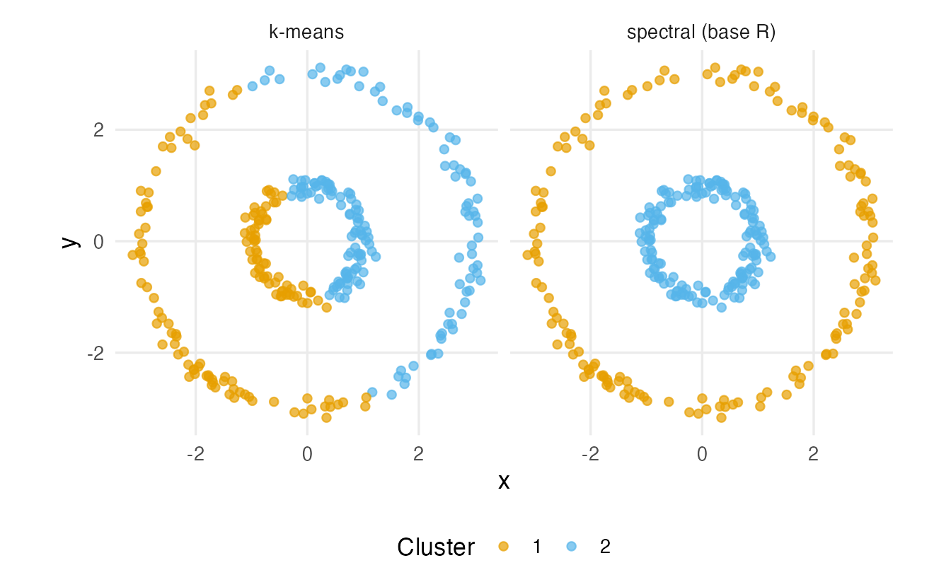

Figure 1: Concentric rings. Left: k-means slices them. Right: spectral clustering (our base-R implementation) follows the rings.

NoteGoing deeper: the graph Laplacian and why eigenvectors find clusters

For a weighted graph with affinity matrix \(A\) and degree matrix \(D\), the graph Laplacian is \(L = D - A\) and the symmetric normalised Laplacian is

\[ L_{\text{sym}} = I - D^{-1/2} A D^{-1/2} = I - M . \]

So \(M\) and \(L_{\text{sym}}\) have the same eigenvectors, and eigenvalue \(\mu\) of \(M\) corresponds to eigenvalue \(\lambda = 1 - \mu\) of \(L_{\text{sym}}\). The eigenvalues returned by spectral_embed() are these \(\lambda\)’s, in increasing order. Key facts:

• \(L\) is positive semi-definite: for any vector \(f\), \(f^\top L f = \tfrac12 \sum_{i,j} A_{ij} (f_i - f_j)^2 \ge 0\). A small value means that \(f\) changes little between strongly connected points.
• The eigenvalue \(0\) of \(L_{\text{sym}}\) has multiplicity equal to the number of connected components of the graph; its eigenspace is spanned by \(D^{1/2}\mathbf{1}_{C}\) for each component \(C\) (indicator vectors, reweighted by \(\sqrt{d_i}\)).
• So if the graph has \(k\) separate pieces, the \(k\) leading eigenvectors of \(M\) are (up to rotation) indicator vectors of the pieces. After normalising the rows, all points of a piece map to the same point on the unit sphere — exactly what we saw for the rings.
• When the pieces are weakly (not completely) connected, perturbation theory says the embedding is close to that ideal, and k-means in the embedding still separates them. Formally, the method solves a continuous relaxation of the normalised cut problem: split the graph so that the total weight of edges cut, relative to the volume of each side, is minimal (Shi & Malik, 2000; von Luxburg, 2007).

A quick numerical check of the second fact on the rings: the first two Laplacian eigenvalues are practically 0, the third is not.

signif(emb_rings$eigenvalues[1:4], 2)

#> [1] 5.6e-16 1.6e-09 1.4e-03 4.7e-03

5. Choosing the scale s

The scale is the most important choice in spectral clustering. Let us try a range of values, from much smaller to much larger than the kNN heuristic.

s_grid <- s_rings * c(0.5, 0.75, 1, 1.5, 2, 4, 10)
scale_res <- tibble(s = s_grid) |>
  mutate(
    cl  = lapply(s, \(v) { set.seed(1); spectral_cluster(X_rings, 2, v) }),
    ari_truth = sapply(cl, \(c1) adjustedRandIndex(c1, rings$truth)),
    lambda_2  = sapply(s, \(v) spectral_embed(X_rings, v, 2)$eigenvalues[2]),
    lambda_3  = sapply(s, \(v) spectral_embed(X_rings, v, 2)$eigenvalues[3])
  )
scale_res |> select(-cl) |> mutate(across(everything(), \(v) signif(v, 2)))

#> # A tibble: 7 × 4
#>       s ari_truth  lambda_2 lambda_3
#>   <dbl>     <dbl>     <dbl>    <dbl>
#> 1  0.14    1      0         0.000056
#> 2  0.2     1      8.2  e-15 0.00052 
#> 3  0.27    1      1.600e- 9 0.0014  
#> 4  0.41    1      4.300e- 5 0.0043  
#> 5  0.54    1      3.5  e- 3 0.011   
#> 6  1.1     0.21   2.2  e- 1 0.3     
#> 7  2.7     0.0054 7.1  e- 1 0.76

TipHow to read this output

• For a wide range of scales around the heuristic (here from half to twice \(s\)), the result is the same and correct: the method is stable in \(s\). That plateau is what we want to see.
• When \(s\) becomes comparable with the gap between the rings, links across the gap get real weight, \(\lambda_2\) is no longer close to 0, and the result degrades towards the k-means answer.
• A very common alternative heuristic, the median of all pairwise distances (median(dist(x)) = 2.71 here), is close to the last row of the table — far too wide for these data. Global distances describe the size of the whole data cloud, not the size of a neighbourhood.
• (Very small scales cause the opposite problem: the graph breaks into many little pieces, several eigenvalues are 0, and the eigenvectors describe arbitrary fragments.)

Do not choose s with the silhouette

It is tempting to try many values of \(s\) and keep the one with the best average silhouette, as the old version of this lesson did. Look at what happens:

d_rings <- dist(X_rings)
scale_res |>
  mutate(silhouette = sapply(cl, \(c1) mean(silhouette(c1, d_rings)[, 3]))) |>
  select(s, ari_truth, silhouette) |>
  mutate(across(everything(), \(v) round(v, 3)))

#> # A tibble: 7 × 3
#>       s ari_truth silhouette
#>   <dbl>     <dbl>      <dbl>
#> 1 0.135     1          0.198
#> 2 0.203     1          0.198
#> 3 0.27      1          0.198
#> 4 0.405     1          0.198
#> 5 0.541     1          0.198
#> 6 1.081     0.21       0.374
#> 7 2.703     0.005      0.339

The silhouette, computed with Euclidean distances in the original space, is higher for the wrong answer. It rewards compact, convex, well-separated clusters (see the introduction) — exactly the assumption that spectral clustering is meant to drop. Choosing \(s\) by silhouette pushes spectral clustering back towards k-means. Use the eigengap and stability instead.

6. Choosing k: the eigengap

The Laplacian eigenvalues also suggest the number of clusters. If the graph consists of \(k\) nearly-separate pieces, the first \(k\) eigenvalues are close to 0 and the \((k+1)\)-th is clearly larger. This jump is the eigengap.

tibble(index = 1:10, lambda = emb_rings$eigenvalues[1:10]) |>
  ggplot(aes(index, pmax(lambda, 1e-12))) +
  geom_point(size = 2.5, colour = "#0072B2") +
  geom_line(colour = "#0072B2") +
  scale_x_continuous(breaks = 1:10) +
  scale_y_log10() +
  labs(x = "Index", y = "Laplacian eigenvalue (log scale)")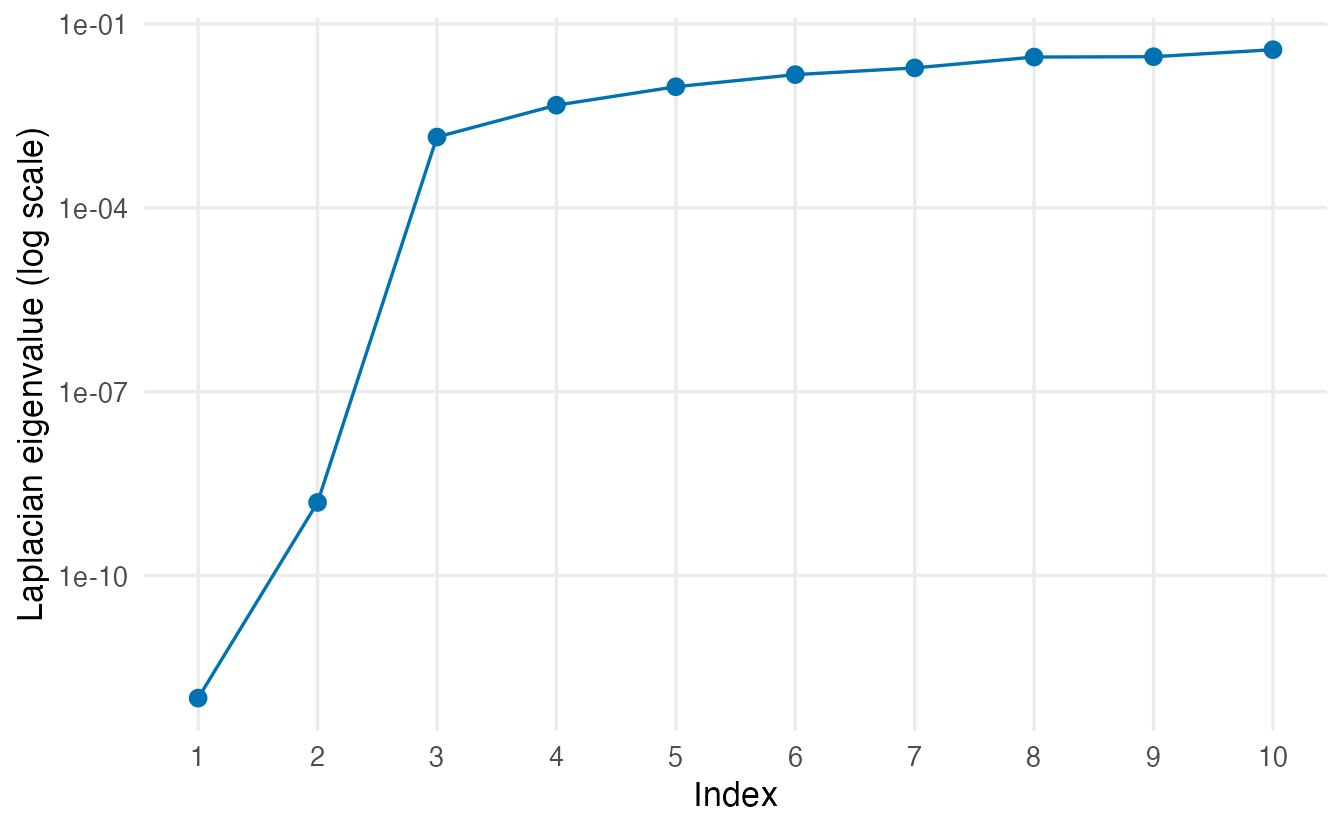

Figure 2: First 10 eigenvalues of the normalised Laplacian for the rings (log scale; values below 1e-12 are drawn at 1e-12). Two eigenvalues are essentially zero, then there is a jump.

For the rings the second eigenvalue is about 2^{-9} and the third about 0.001: a jump of several orders of magnitude after \(k = 2\). Two practical remarks:

• Look at the eigenvalues on a log scale or as ratios when they are tiny. Long thin clusters such as rings have many small (but non-zero) eigenvalues inside each cluster; on a linear scale the differences between them can look larger than the crucial jump from “zero” to “small”.
• The eigengap depends on \(s\). Read it for a scale at which the clustering is stable.

7. kernlab::specc()

The kernlab package implements the same algorithm in specc(). Its RBF kernel is parametrised differently:

\[ \texttt{rbfdot(sigma)}: \quad k(x, y) = \exp\!\left(-\sigma \lVert x - y\rVert^2\right), \]

so sigma is an inverse squared width: larger sigma means narrower neighbourhoods. Comparing with our affinity, \(\sigma = 1/(2s^2)\).

sigma_rings <- 1 / (2 * s_rings^2)
sigma_rings

#> [1] 6.844

set.seed(1)
sc_rings <- specc(X_rings, centers = 2, kernel = "rbfdot",
                  kpar = list(sigma = sigma_rings))
cl_specc <- as.vector(sc_rings@.Data)
table(specc = cl_specc, ours = cl_sp)

#>      ours
#> specc   1   2
#>     1 150   0
#>     2   0 150

adjustedRandIndex(cl_specc, rings$truth)

#> [1] 1

specc() returns an object that behaves like a vector of cluster labels (@.Data), with extra information available through size(sc), centers(sc) (centres in the embedding) and kernelf(sc) (the kernel used).

By default, kpar = "automatic" lets specc() estimate sigma from the data with its own heuristic:

set.seed(1)
sc_auto <- specc(X_rings, centers = 2)
kernelf(sc_auto)

#> Gaussian Radial Basis kernel function. 
#>  Hyperparameter : sigma =  15.570469094623

adjustedRandIndex(as.vector(sc_auto@.Data), rings$truth)

#> [1] 1

The automatic choice gives an ARI of 1 here. Whatever value is used, check it: convert it back to a width, \(s = 1/\sqrt{2\sigma}\), and compare it with the distances in your data. (kpar = "local" uses a different, local scale for each point, following Zelnik-Manor & Perona, 2004.)

8. Real data: the wholesale customers

Spectral clustering is designed for non-convex, connected shapes. Do the wholesale data have them? Same preprocessing as before:

wholesale <- read_csv(data_path("wholesale_customers.csv"),
                      show_col_types = FALSE)
spend_vars <- c("Fresh", "Milk", "Grocery", "Frozen",
                "Detergents_Paper", "Delicassen")

X <- wholesale |>
  select(all_of(spend_vars)) |>
  mutate(across(everything(), log1p)) |>
  scale()

s_w <- knn_scale(X)
emb_w <- spectral_embed(X, s_w, k = 2)
round(emb_w$eigenvalues[1:8], 3)

#> [1] 0.000 0.231 0.399 0.488 0.565 0.594 0.608 0.649

tibble(index = 1:10, lambda = emb_w$eigenvalues[1:10]) |>
  ggplot(aes(index, lambda)) +
  geom_point(size = 2.5, colour = "#0072B2") +
  geom_line(colour = "#0072B2") +
  scale_x_continuous(breaks = 1:10) +
  labs(x = "Index", y = "Laplacian eigenvalue")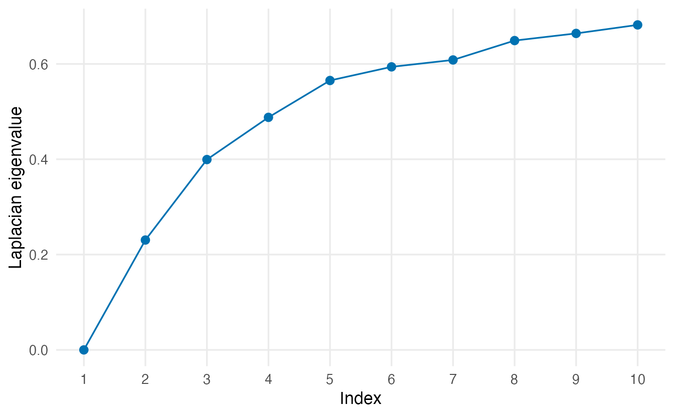

Figure 3: First 10 Laplacian eigenvalues for the wholesale data. After the first (always 0), they grow smoothly: there is no group of near-zero eigenvalues and no clear eigengap.

Only the first eigenvalue is 0; the second is already 0.23. The similarity graph is one connected piece with no weakly linked parts: the eigengap gives no evidence for separate groups. This agrees with what DBSCAN told us in the previous lessons. If we still want a two-group segmentation, we can compute it and compare:

set.seed(1)
cl_w <- spectral_cluster(X, k = 2, s = s_w)

set.seed(1)
sc_w <- specc(X, centers = 2, kernel = "rbfdot",
              kpar = list(sigma = 1 / (2 * s_w^2)))

set.seed(123)
km_w <- kmeans(X, centers = 2, nstart = 50)

c(ours_vs_specc    = adjustedRandIndex(cl_w, as.vector(sc_w@.Data)),
  ours_vs_kmeans   = adjustedRandIndex(cl_w, km_w$cluster),
  ours_vs_channel  = adjustedRandIndex(cl_w, wholesale$Channel),
  kmeans_vs_channel = adjustedRandIndex(km_w$cluster, wholesale$Channel))

#>     ours_vs_specc    ours_vs_kmeans   ours_vs_channel kmeans_vs_channel 
#>            1.0000            0.9284            0.5135            0.5135

Stability across scales

tibble(mult = c(0.5, 0.75, 1, 1.5, 2)) |>
  mutate(
    cl = lapply(mult, \(m) { set.seed(1); spectral_cluster(X, 2, m * s_w) }),
    sizes = sapply(cl, \(c1) paste(sort(table(c1)), collapse = "/")),
    ari_vs_s = sapply(cl, \(c1) round(adjustedRandIndex(c1, cl_w), 3))
  ) |>
  select(-cl)

#> # A tibble: 5 × 3
#>    mult sizes   ari_vs_s
#>   <dbl> <chr>      <dbl>
#> 1  0.5  10/430    -0.008
#> 2  0.75 186/254    0.964
#> 3  1    188/252    1    
#> 4  1.5  189/251    0.937
#> 5  2    194/246    0.894

TipHow to read these outputs

• With the kNN scale, our implementation splits the clients into groups of 188 and 252, essentially the same split as k-means (ARI 0.93), and with the same relation to the sales channel (ARI 0.51 versus 0.51 for k-means).
• The partition is stable for scales from about 0.75 to 2 times \(s\). At half the scale the graph starts to fall apart around a few outlying clients, and the “two clusters” become “a handful of outliers versus everybody else” — another sign that there is no strong, connected group structure.
• specc() with the same sigma should agree closely with our implementation (first number); small differences come from the random starts of k-means in the embedding.

pc <- prcomp(X)$x
bind_rows(
  tibble(PC1 = pc[, 1], PC2 = pc[, 2], cluster = factor(cl_w),
         method = "spectral"),
  tibble(PC1 = pc[, 1], PC2 = pc[, 2], cluster = factor(km_w$cluster),
         method = "k-means")
) |>
  ggplot(aes(PC1, PC2, colour = cluster)) +
  geom_point(alpha = 0.6) +
  facet_wrap(~ method) +
  labs(colour = "Cluster")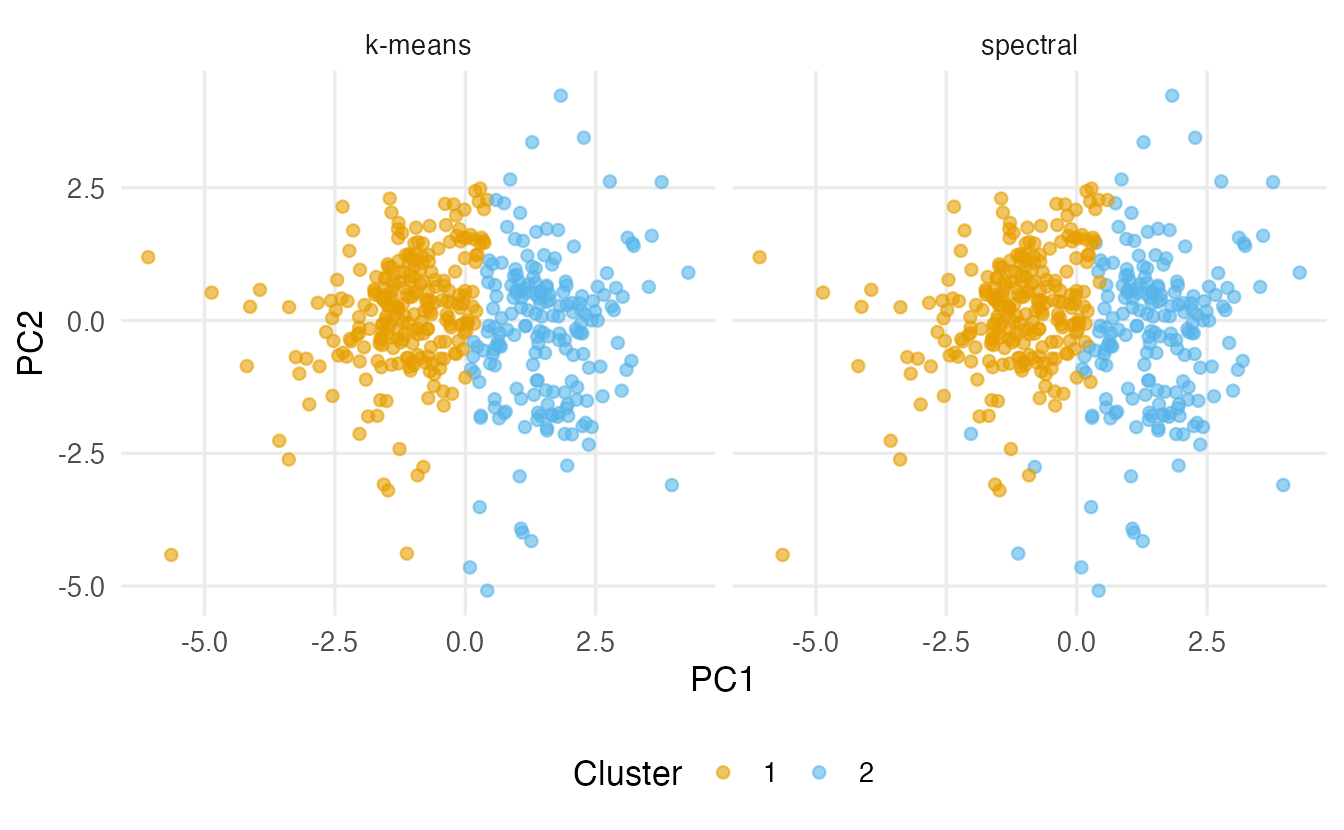

Figure 4: Spectral (left) and k-means (right) partitions of the wholesale clients, on the first two principal components.

Profiles in original units, as always:

wholesale |>
  mutate(cluster = factor(cl_w)) |>
  summarise(n = n(), across(all_of(spend_vars), median), .by = cluster) |>
  arrange(cluster)

#> # A tibble: 2 × 8
#>   cluster     n  Fresh  Milk Grocery Frozen Detergents_Paper Delicassen
#>   <fct>   <int>  <dbl> <dbl>   <dbl>  <dbl>            <dbl>      <dbl>
#> 1 1         252 10348.  1889   2406.   2255              322       774 
#> 2 2         188  5406.  7579  11443    1044             4495      1378.

ImportantAn honest conclusion for the wholesale data

Spectral clustering does not add anything here. The eigenvalues show a single connected cloud, and the two-cluster solution reproduces the k-means split (shop-like versus restaurant-like clients). When the groups are roughly convex blobs — or when there are no clear groups at all — a simpler method is easier to explain and cheaper to compute. Spectral clustering earns its extra complexity when the clusters are non-convex but connected, like the rings.

9. Practical notes

• Cost. The affinity matrix has \(n^2\) entries and a full eigendecomposition costs about \(n^3\) operations: fine for a few thousand points, too slow beyond that. Use sparse \(k\)-nearest-neighbour graphs, the Nyström approximation (specc(..., nystrom.red = TRUE)), or a subsample.
• Scaling. The affinity uses Euclidean distances, so standardise variables measured in different units, exactly as for k-means.
• Outliers. A point far from everybody has tiny affinities and can form its own “cluster”; check cluster sizes.

WarningCommon pitfalls

1. Confusing kernlab’s sigma with a width. In rbfdot(sigma) the kernel is \(\exp(-\sigma\lVert x-y\rVert^2)\): sigma is an inverse squared width, \(\sigma = 1/(2s^2)\). Doubling sigma makes neighbourhoods narrower.
2. Choosing the scale or k by silhouette in the original space. It favours convex clusters and steers spectral clustering back to the k-means answer. Use the eigengap and stability.
3. Using a global scale such as the median of all distances for data with thin or nested structures. Tie the scale to neighbourhood size (kNN distances) and check a range around it.
4. Reading the eigengap on a linear scale only. When eigenvalues are tiny, the decisive jump is in orders of magnitude.
5. Assuming spectral clustering is always better. On blob-like data it reproduces k-means at a much higher cost.
6. Forgetting set.seed(). The final k-means step (and specc()) uses random starts.

10. Check your understanding

NoteQ1. kernlab reports sigma = 2. What is the corresponding scale s in our parametrisation?

\(s = 1/\sqrt{2\sigma} = 1/\sqrt{4} = 0.5\). Points much closer than 0.5 are strongly linked; points more than about 1.5 apart are practically unlinked.

NoteQ2. The first five Laplacian eigenvalues are 0, 0, 0, 0.41, 0.47. How many clusters does the eigengap suggest?

Three: three eigenvalues are (essentially) zero, so the graph has three nearly separate pieces, and the jump comes after the third.

NoteQ3. Why does a ring become a single point in the spectral embedding?

Because, when the graph splits into separate pieces, the leading eigenvectors are constant (up to the \(\sqrt{d_i}\) weights) on each piece. After normalising each row to length 1, all points of the same piece get the same coordinates.

NoteQ4. Spectral clustering and k-means give ARI 0.95 on your data. What do you report?

That the cluster structure, whatever it is, is captured just as well by k-means. Prefer the simpler method for communication, and mention that a graph-based method gave the same answer — a useful robustness check.

11. Exercises

★ Exercise 1 — affinities by hand. With \(s = 0.5\), compute the RBF affinity of two points at distance 0.25, 0.5, 1 and 2. Then give the equivalent kernlab sigma.

TipSolution

d <- c(0.25, 0.5, 1, 2)
round(exp(-d^2 / (2 * 0.5^2)), 4)   # 0.8825 0.6065 0.1353 0.0003
1 / (2 * 0.5^2)                     # sigma = 2

At distance \(s\) the affinity is \(e^{-1/2} \approx 0.61\); at \(4s\) it is practically zero.

★★ Exercise 2 — debug. A student wants wider neighbourhoods than the default and writes specc(X, centers = 2, kpar = list(sigma = 50)), expecting a smoother result. The clustering becomes erratic, with tiny clusters. Why?

TipSolution

In kernlab, sigma multiplies the squared distance: \(\exp(-\sigma\lVert x-y\rVert^2)\). A large sigma means a narrow kernel (\(s = 1/\sqrt{2 \cdot 50} = 0.1\)), so the graph falls apart into fragments and tiny clusters appear. For wider neighbourhoods, decrease sigma.

★★ Exercise 3 — two moons. Generate the two moons of the DBSCAN lesson without the background points (copy the function make_moons() from that lesson, then set.seed(1); moons <- make_moons()). Run spectral_cluster() with the kNN scale and k-means with \(k = 2\), and compare both with the truth. Look at the first six Laplacian eigenvalues.

TipSolution

set.seed(1)
moons <- make_moons()
X_m <- as.matrix(moons[, c("x", "y")])
s_m <- knn_scale(X_m)
set.seed(1)
cl_m <- spectral_cluster(X_m, k = 2, s = s_m)
set.seed(1)
km_m <- kmeans(X_m, centers = 2, nstart = 25)
c(spectral = adjustedRandIndex(cl_m, moons$truth),
  kmeans   = adjustedRandIndex(km_m$cluster, moons$truth))
signif(spectral_embed(X_m, s_m, 2)$eigenvalues[1:6], 2)

Spectral clustering recovers the moons perfectly (ARI 1); k-means does not (about 0.29). The eigenvalues show two values near zero (the second is about \(5 \times 10^{-6}\)) and then a jump to the order of \(10^{-3}\).

★★ Exercise 4 — interpret. A colleague tuned sigma over a grid by maximising the average silhouette and reports: “best sigma = 0.05, silhouette 0.41; spectral clustering agrees with k-means (ARI 0.97)”. What is your comment?

TipSolution

The agreement with k-means is not surprising: a small sigma is a wide kernel, which makes spectral clustering behave like a centroid method, and the silhouette favours exactly the convex, k-means-like partitions. The tuning procedure was biased towards the k-means answer. To know whether spectral clustering finds a different, connected structure, look at the eigengap and at the stability of the partition over a range of scales tied to neighbourhood size.

★★★ Exercise 5 — mini-analysis: penguins. Standardise the four numeric penguins measurements (complete cases). Compute the kNN scale and the first 8 Laplacian eigenvalues. How many clusters does the eigengap suggest? Fit spectral_cluster() with that \(k\) and with \(k = 3\), and compare with the species and with k-means (\(k = 3\)).

TipSolution

peng <- penguins |>
  select(species, bill_len, bill_dep, flipper_len, body_mass) |>
  na.omit()
Xp <- scale(select(peng, -species))
s_p <- knn_scale(Xp)
round(spectral_embed(Xp, s_p, 2)$eigenvalues[1:8], 4)

set.seed(1); cl_p2 <- spectral_cluster(Xp, k = 2, s = s_p)
set.seed(1); cl_p3 <- spectral_cluster(Xp, k = 3, s = s_p)
set.seed(1); km_p  <- kmeans(Xp, centers = 3, nstart = 25)$cluster
table(cl_p2, peng$species)
sapply(list(spectral_2 = cl_p2, spectral_3 = cl_p3, kmeans_3 = km_p),
       \(cl) adjustedRandIndex(cl, peng$species))

There is a clear gap after two eigenvalues (the second is about 0.0005, the third about 0.09): Gentoo penguins are well separated from the others, while Adelie and Chinstrap form one connected cloud. With \(k = 2\) the spectral solution is exactly “Gentoo versus the rest” (ARI about 0.66). Forcing \(k = 3\) splits the Adelie–Chinstrap cloud, and here the split follows the species quite closely (ARI about 0.92, better than about 0.79 for k-means). So the eigengap detects gaps: when two groups touch, it does not see them, even though the method may still separate them well once you ask for three clusters for other reasons (here, prior knowledge of three species).

Summary

Step / idea	Code	Remember
RBF affinity	exp(-dist^2 / (2 * s^2)), zero diagonal	s is a length
Scale heuristic	median distance to the 7th neighbour	check a range around it
Embedding	leading eigenvectors of \(D^{-1/2} A D^{-1/2}\), rows normalised	eigen(M, symmetric = TRUE)
Clustering	kmeans() on the embedding	set.seed(), nstart
Number of clusters	eigengap of the Laplacian eigenvalues	log scale for tiny values
kernlab	specc(x, centers = k, kernel = "rbfdot", kpar = list(sigma = ...))	\(\sigma = 1/(2s^2)\), larger = narrower
Automatic width	specc(x, centers = k); kernelf(sc)	check the value it chose

• Spectral clustering groups points by connectivity in a similarity graph, so it can separate non-convex shapes such as rings and moons.
• It works by turning the graph into an embedding with a few eigenvectors, where connected groups become compact, and then running k-means there.
• The scale is the critical choice: tie it to neighbourhood size, look for a stable plateau, and read the eigengap to choose \(k\) — never the silhouette in the original space.
• On data without connected, non-convex structure (like the wholesale clients), it reproduces k-means: report that honestly and prefer the simpler method.

NoteFurther reading

• von Luxburg, U. (2007). A tutorial on spectral clustering. Statistics and Computing, 17(4), 395–416. https://doi.org/10.1007/s11222-007-9033-z
• Ng, A., Jordan, M. & Weiss, Y. (2002). On spectral clustering: analysis and an algorithm. Advances in Neural Information Processing Systems 14.
• Karatzoglou, A., Smola, A., Hornik, K. & Zeileis, A. (2004). kernlab — an S4 package for kernel methods in R. Journal of Statistical Software, 11(9). https://doi.org/10.18637/jss.v011.i09