library(dplyr)
library(ggplot2)
library(broom)Simple linear regression
One predictor, one line: fitting, reading and checking a linear model
Understand a regression model as a conditional mean plus noise, fit it by least squares with lm(), read every line of summary(), build confidence and prediction intervals and check the assumptions with diagnostic plots.
NoteLearning objectives
By the end of this lesson you will be able to:
- describe a regression model as a conditional mean plus noise and explain what “least squares” minimises;
- fit a simple regression with
lm()and interpret the slope and intercept in words, with units; - read every line of
summary(lm(...))and connect the slope test tocor.test(); - distinguish a confidence interval for the mean from a prediction interval for a new observation;
- check the assumptions with diagnostic plots and use a log transformation when appropriate.
1. Why do we need a model?
Heavier penguins tend to have longer flippers. A scatterplot shows this at a glance, and the correlation summarises it with a single number. But often we want more:
- How much heavier, on average, is a penguin whose flippers are 10 mm longer?
- If we measure the flipper of a new bird, what body mass should we expect, and how uncertain is that guess?
- Is the relationship strong enough that it is unlikely to be an accident of sampling?
A regression model answers all three. It describes how the average of a response variable \(y\) changes as a predictor \(x\) changes, and how much individual observations scatter around that average.
2. A model is “conditional mean + noise”
Let us look at the penguins. For each band of flipper lengths, the orange points show the mean body mass of the birds in that band.
ggplot(penguins, aes(flipper_len, body_mass)) +
  geom_point(alpha = 0.3) +
  stat_summary_bin(fun = mean, bins = 12, geom = "point",
                   colour = "#E69F00", size = 3) +
  labs(x = "Flipper length (mm)", y = "Body mass (g)")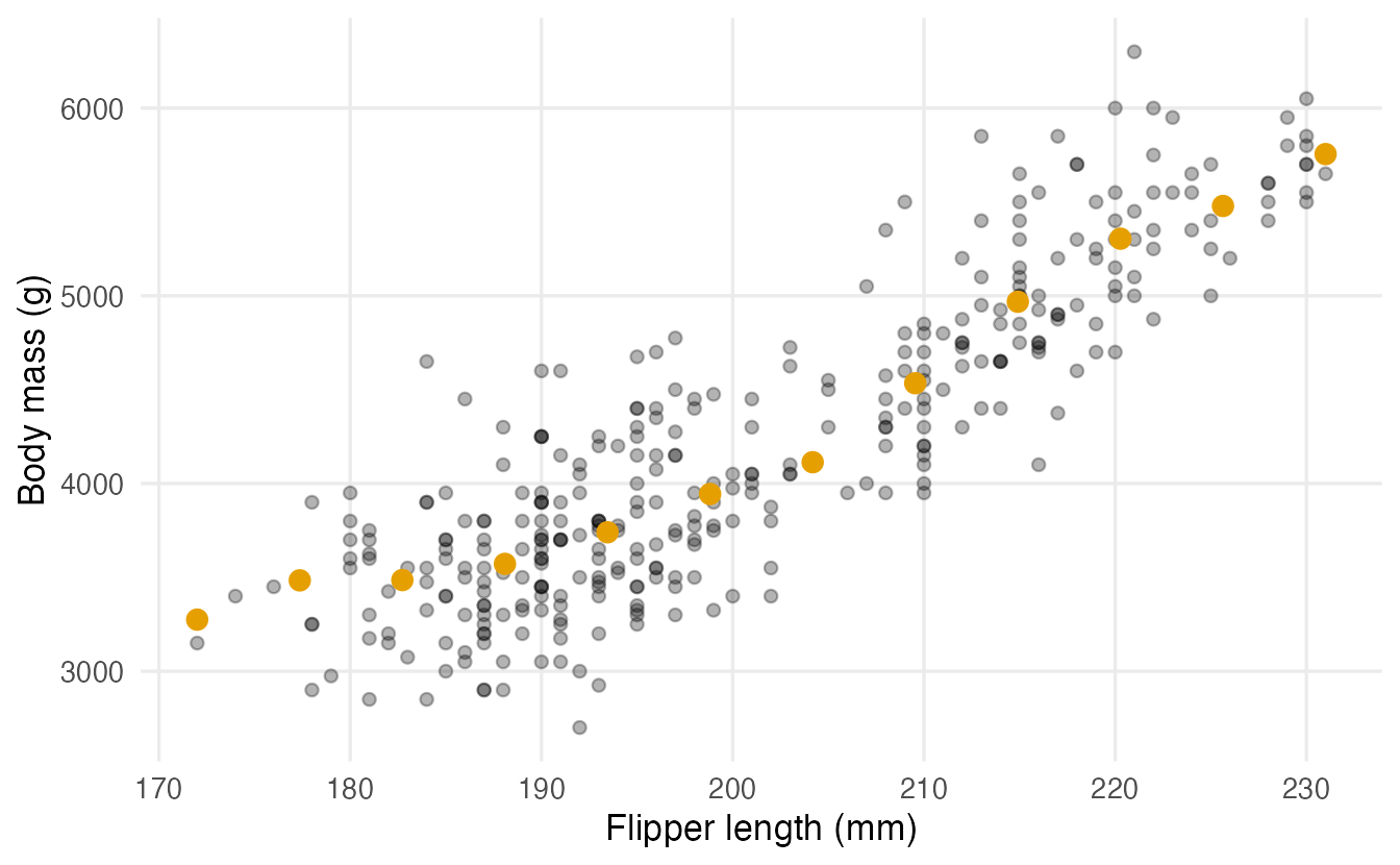
The band means climb almost along a straight line. That line is the conditional mean: the average of \(y\) given a value of \(x\). The individual birds do not sit on the line — they scatter around it. This scatter is the noise (or error): everything about body mass that flipper length does not explain (sex, species, diet, measurement error…).
So a simple linear regression says:
\[ \underbrace{y_i}_{\text{observed}} \;=\; \underbrace{\beta_0 + \beta_1 x_i}_{\text{conditional mean}} \;+\; \underbrace{\varepsilon_i}_{\text{noise}} \]
- \(\beta_0\), the intercept: the mean of \(y\) when \(x = 0\);
- \(\beta_1\), the slope: how much the mean of \(y\) changes when \(x\) increases by one unit;
- \(\varepsilon_i\): the deviation of observation \(i\) from the line, assumed to average zero.
The Greek letters are population parameters — unknown. From the data we compute estimates \(\hat\beta_0\) and \(\hat\beta_1\) (read “beta-hat”).
3. Least squares: which line is “best”?
We start with a tiny dataset that ships with R: women contains the average height (inches) and weight (pounds) of American women aged 30–39, for 15 heights.
For any candidate line, the residual of a point is its vertical distance from the line: observed \(y\) minus the \(y\) predicted by the line. The plot shows the residuals (red segments) for the line R will choose.
m_women <- lm(weight ~ height, data = women)

augment(m_women) |>
  ggplot(aes(height, weight)) +
  geom_segment(aes(xend = height, yend = .fitted), colour = "#D55E00") +
  geom_abline(intercept = coef(m_women)[1], slope = coef(m_women)[2]) +
  geom_point(size = 2) +
  labs(x = "Height (in)", y = "Weight (lb)")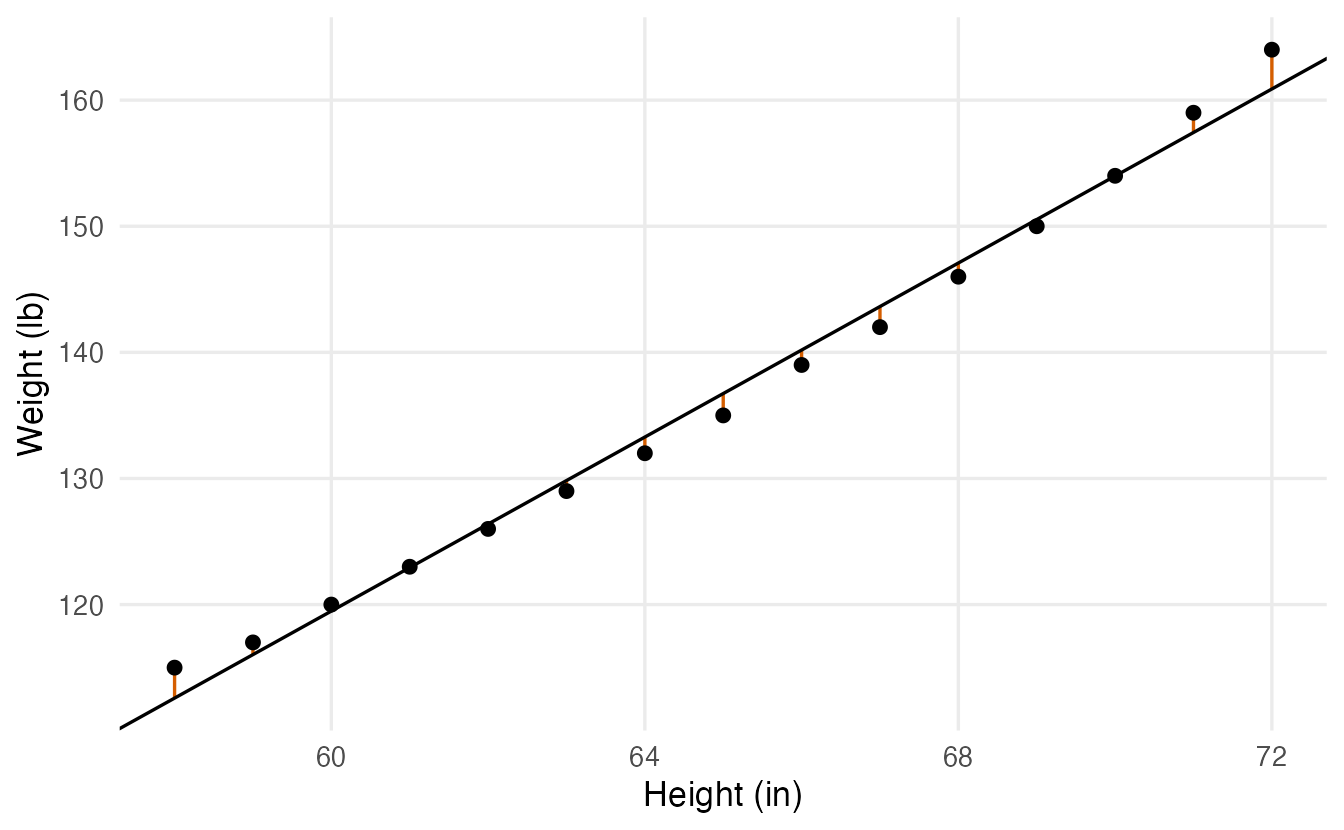
Ordinary least squares (OLS) picks the line that makes the sum of squared residuals (RSS, residual sum of squares) as small as possible. Squaring makes all residuals positive and penalises large misses heavily. Let us compute the RSS for a few candidate slopes (each line passes through the point of means, as the OLS line always does):
rss <- function(b0, b1) sum((women$weight - (b0 + b1 * women$height))^2)

slopes <- c(3, 3.2, 3.45, 3.7, 4)
intercepts <- mean(women$weight) - slopes * mean(women$height)
data.frame(slope = slopes, RSS = mapply(rss, intercepts, slopes))
#> slope RSS
#> 1 3.00 86.93
#> 2 3.20 47.73
#> 3 3.45 30.23
#> 4 3.70 47.73
#> 5 4.00 114.93The RSS is smallest at a slope of 3.45 and grows on either side. No other straight line has a smaller RSS.
OLS by hand vs lm()
For one predictor the minimisation has a closed-form answer: the slope is the covariance of \(x\) and \(y\) divided by the variance of \(x\), and the intercept makes the line pass through \((\bar x, \bar y)\).
b1 <- cov(women$height, women$weight) / var(women$height)
b0 <- mean(women$weight) - b1 * mean(women$height)
c(intercept = b0, slope = b1)
#> intercept slope
#> -87.52 3.45coef(m_women)#> (Intercept) height
#> -87.52 3.45lm() (“linear model”) gives the same numbers. The formula weight ~ height reads “weight modelled by height”: the response goes on the left of ~, the predictor on the right.
NoteGoing deeper: deriving the OLS estimates
We minimise \(\text{RSS}(b_0, b_1) = \sum_i (y_i - b_0 - b_1 x_i)^2\). Setting both partial derivatives to zero gives the normal equations
\[ \sum_i (y_i - b_0 - b_1 x_i) = 0, \qquad \sum_i x_i (y_i - b_0 - b_1 x_i) = 0 . \]
The first says the residuals sum to zero, so \(\hat\beta_0 = \bar y - \hat\beta_1 \bar x\). Substituting into the second,
\[ \hat\beta_1 = \frac{\sum_i (x_i - \bar x)(y_i - \bar y)}{\sum_i (x_i - \bar x)^2} = \frac{\operatorname{cov}(x, y)}{\operatorname{var}(x)} = r \,\frac{s_y}{s_x}, \]
where \(r\) is the Pearson correlation and \(s_x, s_y\) the standard deviations. Under the assumptions of Section 9, OLS is the best linear unbiased estimator (Gauss–Markov theorem): no other unbiased estimator that is linear in \(y\) has a smaller variance.
4. Interpreting slope and intercept in words
The slope is 3.45: for each additional inch of height, average weight is 3.45 pounds higher. Always say it with units, and say “on average” — individual women do not gain weight by growing an inch; we are comparing groups of women who differ by one inch in height.
The intercept is -87.5 pounds: the predicted weight of a woman 0 inches tall. That is nonsense — not because the model is wrong, but because \(x = 0\) is far outside the data (heights go from 58 to 72 in). A common fix is to centre the predictor, so that the intercept refers to a meaningful value:
lm(weight ~ I(height - 65), data = women) |> coef()#> (Intercept) I(height - 65)
#> 136.73 3.45Now the intercept, 136.7, is the predicted weight at 65 inches. The slope is unchanged. (I() tells the formula to compute height - 65 arithmetically.)
5. Reading summary(lm) line by line
Back to penguins. We model body mass from flipper length:
m_peng <- lm(body_mass ~ flipper_len, data = penguins)
summary(m_peng)
#>
#> Call:
#> lm(formula = body_mass ~ flipper_len, data = penguins)
#>
#> Residuals:
#> Min 1Q Median 3Q Max
#> -1058.8 -259.3 -26.9 247.3 1288.7
#>
#> Coefficients:
#> Estimate Std. Error t value Pr(>|t|)
#> (Intercept) -5780.83 305.81 -18.9 <2e-16 ***
#> flipper_len 49.69 1.52 32.7 <2e-16 ***
#> ---
#> Signif. codes: 0 '***' 0.001 '**' 0.01 '*' 0.05 '.' 0.1 ' ' 1
#>
#> Residual standard error: 394 on 340 degrees of freedom
#> (2 osservazioni eliminate a causa di valori mancanti)
#> Multiple R-squared: 0.759, Adjusted R-squared: 0.758
#> F-statistic: 1.07e+03 on 1 and 340 DF, p-value: <2e-16
TipHow to read this output
- Call — the model you fitted.
- Residuals — a five-number summary of the residuals. They should be roughly symmetric around 0 (median close to 0, Q1 and Q3 of similar size).
- Coefficients table, one row per parameter:
Estimate— \(\hat\beta\). Penguins with 1 mm longer flippers are on average 49.7 g heavier (about 500 g per 10 mm).Std. Error— how much the estimate would vary from sample to sample: 1.52 g/mm.t value— estimate / standard error: the slope is 32.7 standard errors away from 0. The same signal-to-noise idea as in the t-test.Pr(>|t|)— the p-value for \(H_0: \beta = 0\) (“no linear relationship”). Here it is astronomically small.
- Residual standard error — the typical size of a residual: individual birds are typically about 390 g away from the line. The degrees of freedom are \(n - 2\) (two parameters estimated).
(2 observations deleted due to missingness)—lm()silently drops rows withNAin any variable of the model. Always check this line.- Multiple R-squared — the share of the variance of body mass “explained” by the line: 76%. Adjusted R² penalises extra predictors (useful in the next lesson).
- F-statistic — tests whether the model as a whole beats a model with only an intercept. With one predictor it is just \(t^2\) (1070.7) and has the same p-value.
Confidence intervals for the coefficients come from confint():
confint(m_peng)#> 2.5 % 97.5 %
#> (Intercept) -6382.4 -5179.30
#> flipper_len 46.7 52.67We are 95% confident that, in the population of penguins these birds represent, each extra millimetre of flipper corresponds to between 46.7 and 52.7 g of extra average mass.
NoteGoing deeper: standard error, R² and F
With \(\hat\sigma^2 = \text{RSS}/(n-2)\) (the square of the residual standard error),
\[ \operatorname{SE}(\hat\beta_1) = \frac{\hat\sigma}{\sqrt{\sum_i (x_i - \bar x)^2}}, \qquad t = \frac{\hat\beta_1}{\operatorname{SE}(\hat\beta_1)} \sim t_{n-2} \text{ under } H_0 . \]
The slope is estimated more precisely when the noise \(\hat\sigma\) is small and when the \(x\) values are spread out.
With \(\text{TSS} = \sum_i (y_i - \bar y)^2\) (total sum of squares),
\[ R^2 = 1 - \frac{\text{RSS}}{\text{TSS}}, \qquad F = \frac{(\text{TSS} - \text{RSS})/1}{\text{RSS}/(n-2)} . \]
In simple regression \(R^2 = r^2\), the squared Pearson correlation, and \(F = t^2\).
6. Slope test = correlation test
In the correlation lesson we tested \(H_0: \rho = 0\) with cor.test(). Compare:
ct <- cor.test(penguins$body_mass, penguins$flipper_len)
c(t_cor = unname(ct$statistic), t_slope = s_peng$coefficients[2, 3])
#> t_cor t_slope
#> 32.72 32.72c(r_squared = unname(ct$estimate^2), R2 = s_peng$r.squared)#> r_squared R2
#> 0.759 0.759The two t statistics are identical, and \(r^2 = R^2\). Testing “slope = 0” and testing “correlation = 0” are the same test. The difference is in what you report: the correlation is unit-free and symmetric in \(x\) and \(y\); the slope has units (g per mm) and a direction (predict \(y\) from \(x\)). The slope is the correlation rescaled: \(\hat\beta_1 = r \, s_y / s_x\).
7. Tidy model output with broom
summary() prints nicely but is awkward to reuse. The broom package turns models into data frames:
tidy(m_peng, conf.int = TRUE) # one row per coefficient#> # A tibble: 2 × 7
#> term estimate std.error statistic p.value conf.low conf.high
#> <chr> <dbl> <dbl> <dbl> <dbl> <dbl> <dbl>
#> 1 (Intercept) -5781. 305.8 -18.90 5.587e- 55 -6382. -5179.
#> 2 flipper_len 49.69 1.518 32.72 4.371e-107 46.70 52.67glance(m_peng) # one row per model#> # A tibble: 1 × 12
#> r.squared adj.r.squared sigma statistic p.value df logLik AIC BIC
#> <dbl> <dbl> <dbl> <dbl> <dbl> <dbl> <dbl> <dbl> <dbl>
#> 1 0.7590 0.7583 394.3 1071. 4.371e-107 1 -2528. 5063. 5074.
#> # ℹ 3 more variables: deviance <dbl>, df.residual <int>, nobs <int>augment(m_peng) |> head(4) # one row per observation#> # A tibble: 4 × 9
#> .rownames body_mass flipper_len .fitted .resid .hat .sigma .cooksd
#> <chr> <int> <int> <dbl> <dbl> <dbl> <dbl> <dbl>
#> 1 1 3750 181 3212. 537.7 0.008806 393.8 0.008337
#> 2 2 3800 186 3461. 339.3 0.006223 394.4 0.002334
#> 3 3 3250 195 3908. -657.9 0.003443 393.2 0.004826
#> 4 5 3450 193 3808. -358.5 0.003853 394.4 0.001605
#> # ℹ 1 more variable: .std.resid <dbl>augment() adds .fitted (the point on the line), .resid (the residual) and diagnostic columns (.hat, .cooksd, .std.resid) that we use in Multiple regression.
8. Confidence interval vs prediction interval
Two different questions about a penguin with 200 mm flippers:
- What is the average body mass of all penguins with 200 mm flippers? → confidence interval for the mean.
- What will the body mass of the next penguin with 200 mm flippers be? → prediction interval for one new observation.
new_birds <- data.frame(flipper_len = c(180, 200, 220))
predict(m_peng, newdata = new_birds, interval = "confidence")
#> fit lwr upr
#> 1 3163 3087 3238
#> 2 4156 4114 4198
#> 3 5150 5079 5221predict(m_peng, newdata = new_birds, interval = "prediction")#> fit lwr upr
#> 1 3163 2383 3942
#> 2 4156 3380 4933
#> 3 5150 4371 5929The point prediction is the same (4156 g at 200 mm), but the intervals are very different: about ±42 g for the mean, about ±777 g for a single bird. The prediction interval must also include the bird-to-bird scatter \(\sigma\), which does not shrink when we collect more data.
grid <- data.frame(flipper_len = seq(172, 231, length.out = 100))
bands <- cbind(
  grid,
  predict(m_peng, grid, interval = "confidence") |>
    as.data.frame() |> rename(ci_lwr = lwr, ci_upr = upr),
  predict(m_peng, grid, interval = "prediction") |>
    as.data.frame() |> select(pi_lwr = lwr, pi_upr = upr)
)

ggplot(bands, aes(flipper_len)) +
  geom_ribbon(aes(ymin = pi_lwr, ymax = pi_upr), fill = "#56B4E9",
              alpha = 0.25) +
  geom_ribbon(aes(ymin = ci_lwr, ymax = ci_upr), fill = "#0072B2",
              alpha = 0.5) +
  geom_point(data = penguins, aes(y = body_mass), alpha = 0.3) +
  geom_line(aes(y = fit), linewidth = 1) +
  labs(x = "Flipper length (mm)", y = "Body mass (g)")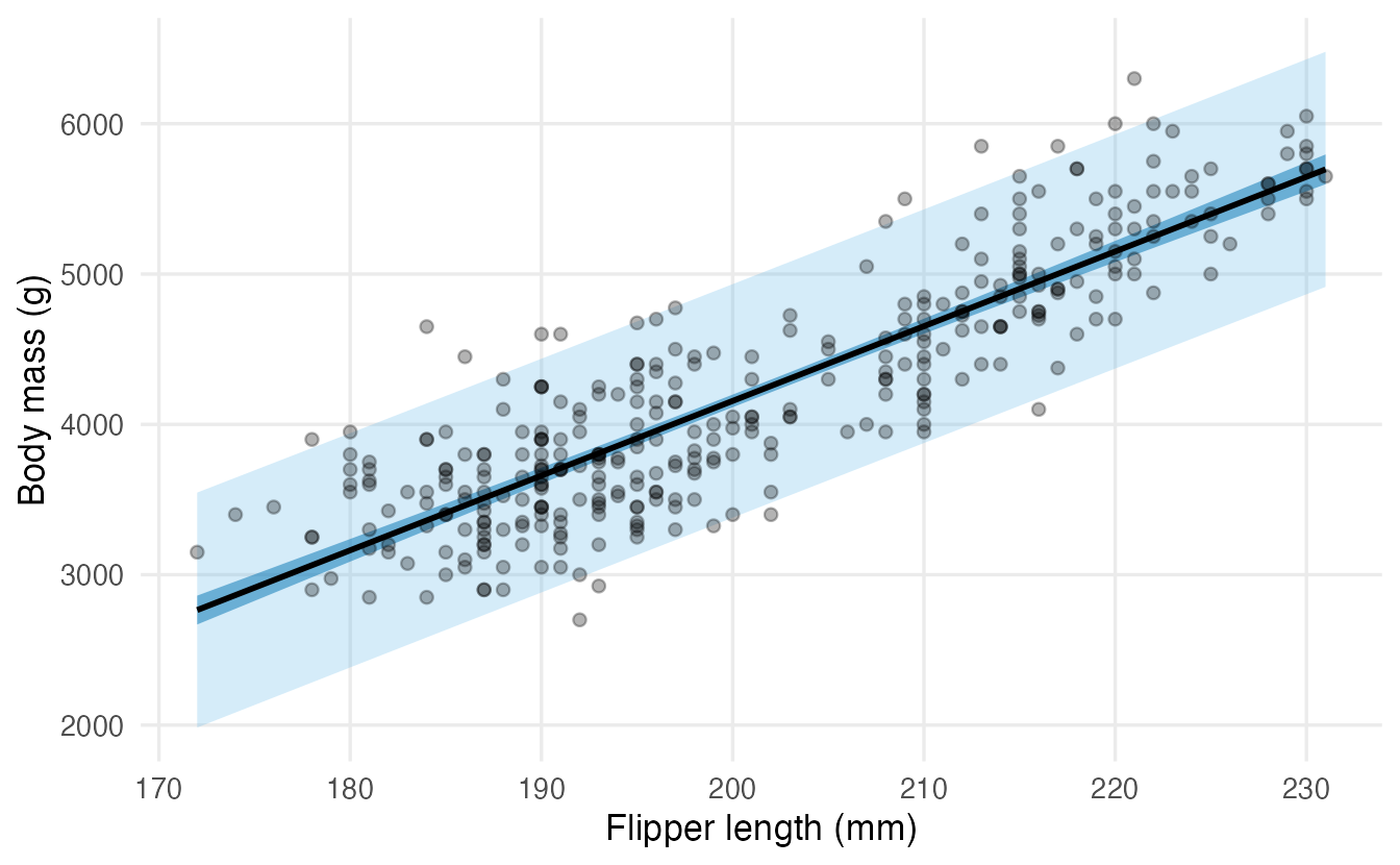
The confidence band is narrow in the middle and widens towards the edges, where we have fewer data. About 95% of the birds fall inside the prediction band. geom_smooth(method = "lm") draws only the confidence band.
NoteGoing deeper: the two standard errors
At a new value \(x_0\), with \(\hat y_0 = \hat\beta_0 + \hat\beta_1 x_0\):
\[ \operatorname{SE}_{\text{mean}} = \hat\sigma\sqrt{\frac1n + \frac{(x_0 - \bar x)^2}{\sum_i (x_i - \bar x)^2}}, \qquad \operatorname{SE}_{\text{pred}} = \hat\sigma\sqrt{1 + \frac1n + \frac{(x_0 - \bar x)^2}{\sum_i (x_i - \bar x)^2}} . \]
Both intervals are \(\hat y_0 \pm t_{n-2,\,0.975} \times \text{SE}\). As \(n \to \infty\) the first SE goes to 0, the second goes to \(\hat\sigma\).
9. Assumptions and diagnostic plots
The estimates are just a best-fitting line; the standard errors, p-values and intervals rely on assumptions. A handy mnemonic is LINE:
| Letter | Assumption | What goes wrong if it fails | How to look |
|---|---|---|---|
| L | Linearity: the conditional mean is a straight line in \(x\) | the line is systematically wrong in places | residuals vs fitted |
| I | Independence of the errors | SEs too small (e.g. repeated measures, time series) | think about the design |
| N | Normality of the errors | matters for small \(n\) and for prediction intervals | normal QQ-plot |
| E | Equal variance (homoscedasticity) | SEs and prediction intervals are wrong | scale-location plot |
Base R draws the four standard diagnostic plots with plot() on the model:
par(mfrow = c(2, 2))
plot(m_peng)
par(mfrow = c(1, 1))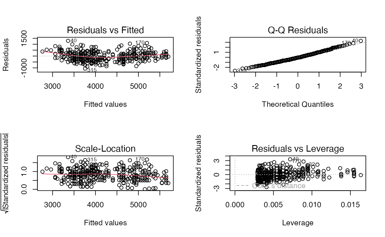
TipHow to read these plots
- Residuals vs Fitted (top left): we want a shapeless cloud around 0 with a flat red line. A curve means the linear form misses something.
- Q-Q Residuals (top right): points on the dashed line mean approximately normal residuals. Curved tails indicate skewness or heavy tails.
- Scale-Location (bottom left): a flat red line means constant spread. A rising line (“funnel”) means the variance grows with the mean.
- Residuals vs Leverage (bottom right): flags observations that pull the line strongly. Points beyond the dashed Cook’s distance contours deserve a closer look (see Multiple regression).
For penguins the plots look reasonable, but the residuals hide a structure we can reveal by colouring them by species:
peng_aug <- augment(m_peng,
                    data = tidyr::drop_na(penguins, body_mass, flipper_len))

peng_aug |>
  ggplot(aes(.fitted, .resid, colour = species)) +
  geom_hline(yintercept = 0, linetype = 2) +
  geom_point(alpha = 0.7) +
  labs(x = "Fitted body mass (g)", y = "Residual (g)", colour = NULL)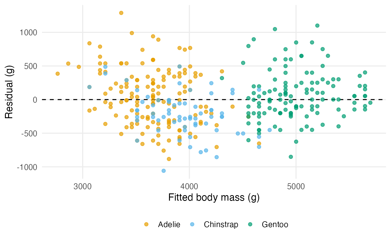
Chinstrap penguins are, on average, 216 g lighter than the line predicts. A missing predictor shows up as structure in the residuals: this is exactly the motivation for multiple regression.
10. Transformations: when the line is curved
Many relationships are multiplicative: doubling one quantity multiplies another by a constant factor. Taking logarithms turns such curves into straight lines. The built-in trees data record the girth (diameter, in inches), height and timber volume of 31 cherry trees.
trees_long <- bind_rows(
  tibble::tibble(scale = "Original scale", x = trees$Girth, y = trees$Volume),
  tibble::tibble(scale = "Log–log scale", x = log(trees$Girth),
                 y = log(trees$Volume))
) |>
  mutate(scale = factor(scale, levels = c("Original scale", "Log–log scale")))

ggplot(trees_long, aes(x, y)) +
  geom_point() +
  geom_smooth(method = "lm", formula = y ~ x, se = FALSE) +
  facet_wrap(~ scale, scales = "free") +
  labs(x = "Girth (in) / log(girth)", y = "Volume (cubic ft) / log(volume)")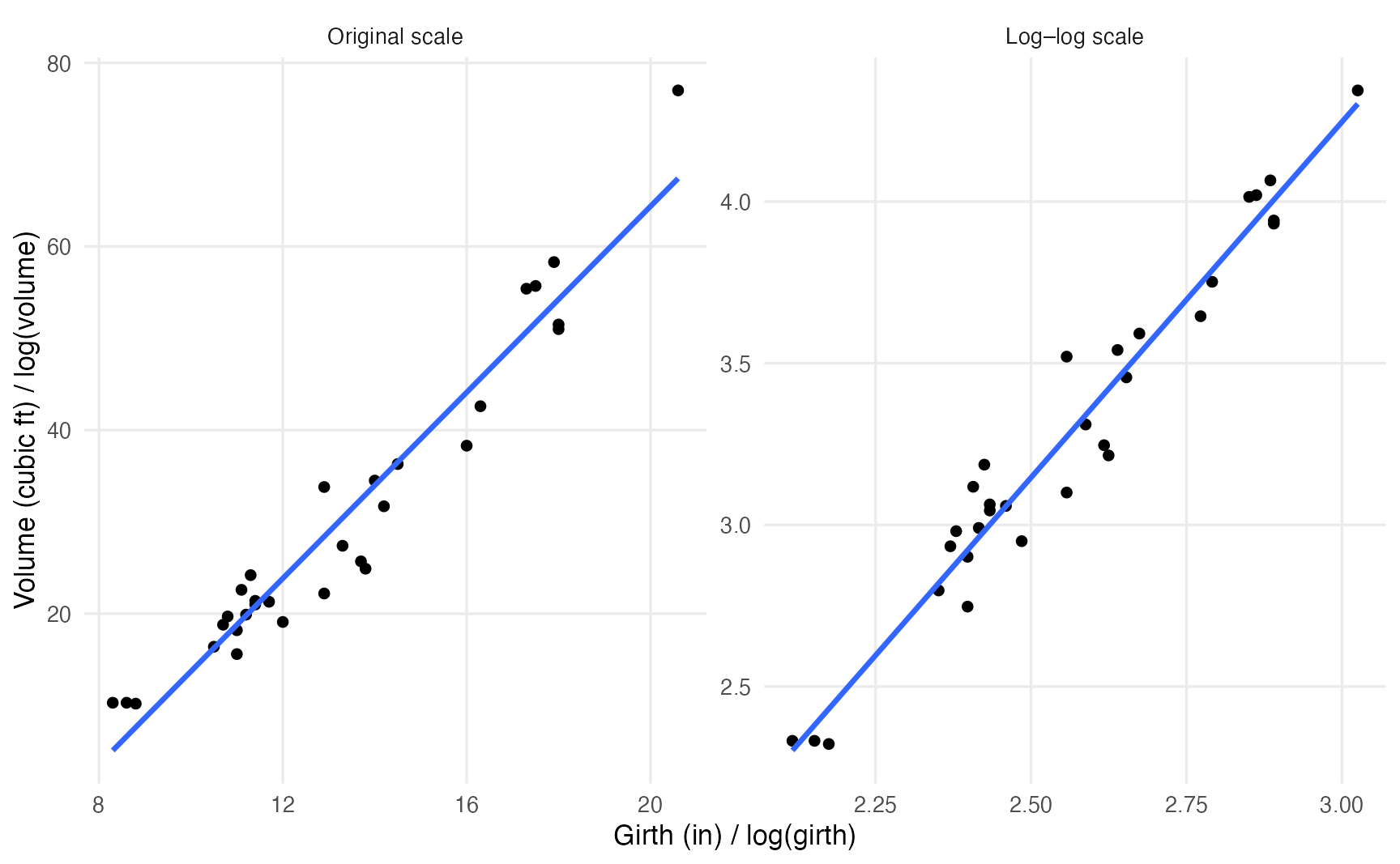
The straight line misses the curvature on the original scale (it is too high in the middle and too low at both ends), but fits well after taking logs.
m_trees <- lm(log(Volume) ~ log(Girth), data = trees)
coef(m_trees)
#> (Intercept) log(Girth)
#> -2.353 2.200On the log–log scale the slope is an elasticity: a 1% larger girth goes with about 2.2% larger volume. (Geometry agrees: volume grows roughly with the square of the diameter.)
When only \(y\) is logged, the slope describes a multiplicative change in \(y\) per unit of \(x\):
m_mpg <- lm(log(mpg) ~ wt, data = mtcars)
exp(coef(m_mpg)["wt"])
#> wt
#> 0.762Each additional 1000 lb of weight multiplies the expected fuel efficiency by 0.76, i.e. about 24% fewer miles per gallon.
| Model | Interpretation of \(\hat\beta_1\) |
|---|---|
| \(y \sim x\) | +1 unit of \(x\) → \(y\) changes by \(\hat\beta_1\) units |
| \(\log y \sim x\) | +1 unit of \(x\) → \(y\) is multiplied by \(e^{\hat\beta_1}\) (≈ \(100\hat\beta_1\)% if small) |
| \(y \sim \log x\) | +1% in \(x\) → \(y\) changes by about \(\hat\beta_1 / 100\) units |
| \(\log y \sim \log x\) | +1% in \(x\) → \(y\) changes by about \(\hat\beta_1\)% |
NoteGoing deeper: back-transforming predictions
If \(\log y = \beta_0 + \beta_1 x + \varepsilon\), then \(\exp(\hat\beta_0 + \hat\beta_1 x)\) estimates the median of \(y\) at \(x\), not the mean. When errors are normal with variance \(\sigma^2\), the mean is \(\exp(\beta_0 + \beta_1 x + \sigma^2/2)\). For small \(\sigma\) the difference is negligible; for noisy data it is not. Prediction intervals, on the other hand, can be back-transformed directly by exponentiating their limits.
11. Regression to the mean
The word “regression” comes from Francis Galton, who noticed that very tall parents tend to have children who are tall, but less extremely tall. This is not a biological force; it happens whenever two measurements are imperfectly correlated. A simulation: 1000 students with a true ability take two tests, each with independent luck.
set.seed(42)
ability <- rnorm(1000, mean = 100, sd = 10)
test1 <- ability + rnorm(1000, sd = 10)
test2 <- ability + rnorm(1000, sd = 10)

top <- test1 > quantile(test1, 0.9)   # top 10% on the first test
c(test1 = mean(test1[top]), test2 = mean(test2[top]))
#> test1 test2
#> 124.4 112.5The best students on test 1 score lower on test 2, on average — nobody got worse; part of their first score was good luck that did not repeat. The slope of test2 on test1 is about 0.49, well below 1. Beware of “treatments” given to the worst performers: they will improve on average even if the treatment does nothing. A control group protects you from this illusion.
WarningCommon pitfalls
- Reading the slope causally. “Growing longer flippers makes a penguin heavier” is not what the model says. The slope compares different birds; without an experiment it describes association, not cause.
- Extrapolating. The line is supported only within the range of the data. The intercept of the
womenmodel (a negative weight at height 0) is an extreme example. - Confusing the confidence and the prediction interval. Use the prediction interval to say where an individual will fall; it is always wider.
- Trusting R² alone. A high R² does not mean the linear form is right (look at the residuals), and a low R² does not mean the slope is unimportant.
- Forgetting the
NAline.lm()drops incomplete rows silently; comparenobs(model)withnrow(data). lm(df$y ~ df$x). Writing the model with$breakspredict()on new data (see Exercise 3). Uselm(y ~ x, data = df).
12. Check your understanding
13. Exercises
★ Exercise 1 — fit and interpret. The built-in cars data give the stopping distance (dist, feet) of cars at different speeds (speed, mph), recorded in the 1920s. Fit dist ~ speed, report the slope with its 95% CI, and write one sentence interpreting it.
TipSolution
m_cars <- lm(dist ~ speed, data = cars)
tidy(m_cars, conf.int = TRUE)
The slope is about 3.9 (95% CI roughly 3.1 to 4.8): cars travelling 1 mph faster needed, on average, about 4 more feet to stop. R² is about 0.65. Note that the intercept (about −17.6 ft at 0 mph) is meaningless — another extrapolation.
★ Exercise 2 — predict the output. Without running it, what will the following code print? Then run it and check.
m <- lm(eruptions ~ waiting, data = faithful)
c(summary(m)$coefficients["waiting", "t value"],
  cor.test(faithful$eruptions, faithful$waiting)$statistic)
TipSolution
Two identical numbers (about 34.1): the t statistic of the slope equals the t statistic of the correlation test. They also share the same p-value.
★★ Exercise 3 — debug. A student wants the predicted weight of a 70-inch woman:
bad <- lm(women$weight ~ women$height)
predict(bad, newdata = data.frame(height = 70))
R prints 15 numbers and a warning instead of one prediction. Why? Fix the code.
TipSolution
The model’s predictor is literally called women$height. newdata contains a column called height, which predict() cannot match, so it falls back to the original data (15 rows) and warns: ‘newdata’ had 1 row but variables found have 15 rows. Use the data = argument:
good <- lm(weight ~ height, data = women)
predict(good, newdata = data.frame(height = 70))   # about 154 lb
★★ Exercise 4 — interpret an output. Using m_peng, a colleague says: “the 95% interval for a penguin with 200 mm flippers is 4114 to 4198 g, so a bird of 4500 g with 200 mm flippers would be very unusual.” Is this right? Compute the appropriate interval and explain.
TipSolution
The colleague used the confidence interval for the mean. For one bird you need the prediction interval:
predict(m_peng, data.frame(flipper_len = 200), interval = "prediction")It runs from about 3380 to 4930 g, so a 4500 g bird is perfectly ordinary. The confidence interval only says where the average of all 200-mm birds is likely to be.
★★★ Exercise 5 — mini-analysis: one species at a time. (a) Fit body_mass ~ flipper_len separately for each of the three species. (b) Compare the three slopes with the slope of the all-species model. (c) Look at R² of the Adelie model. What do you conclude about using a single line for all penguins?
TipSolution
penguins |>
  group_by(species) |>
  group_modify(\(d, key) tidy(lm(body_mass ~ flipper_len, data = d))) |>
  filter(term == "flipper_len")

lm(body_mass ~ flipper_len, data = filter(penguins, species == "Adelie")) |>
  glance()
The within-species slopes are about 33 (Adelie), 35 (Chinstrap) and 55 (Gentoo) g/mm, while the all-species slope is about 50 g/mm. Part of the overall slope comes from the differences between species (Gentoo are both larger-flippered and heavier). Within Adelie, R² drops to about 0.22. One line for all species mixes two things — the within-species relationship and the between-species differences. Multiple regression with species as a predictor separates them.
Summary
| Idea / function | What it does |
|---|---|
lm(y ~ x, data = df) |
fits a linear model by least squares |
coef(), confint() |
estimates and their 95% CIs |
summary() |
estimates, SEs, t, p, residual SE, R², F |
cor.test() |
same test as the slope in simple regression |
tidy(), glance(), augment() |
model output as data frames (broom) |
predict(m, newdata, interval = "confidence") |
interval for the mean response |
predict(m, newdata, interval = "prediction") |
interval for a new observation |
plot(m) |
four diagnostic plots (LINE assumptions) |
lm(log(y) ~ log(x)) |
multiplicative relationships; slope = elasticity |
- A regression model is a conditional mean plus noise; least squares chooses the line with the smallest sum of squared vertical distances.
- Interpret the slope in words, with units and “on average” — and not causally without a design that supports it.
- The p-value of the slope answers “is there a linear association?”; the CI tells you how large it plausibly is.
- Prediction intervals are much wider than confidence intervals.
- Always look at the residuals: patterns there point to missing predictors or a wrong functional form.