Gradient boosting

Many small trees, each one correcting the mistakes of the previous ones

Boosting built from scratch with stumps in base R, the role of learning rate, number of trees, depth and early stopping, pseudo-residuals as the negative gradient of the loss, and tuning XGBoost with tidymodels on the Titanic data.

Level 4 · Models & learning ⏱ ~100 min Prerequisites: Decision trees, Random forests

Learning objectives

By the end of this lesson you will be able to:

explain boosting as fitting small trees sequentially to the residuals of the current model, and implement it from scratch with stumps;
describe how the learning rate, the number of trees, the tree depth and early stopping interact;
define pseudo-residuals as the negative gradient of the loss, and compute them for squared error and log-loss;
specify and tune an XGBoost model with boost_tree() in tidymodels, and read its variable importance;
recognise the main XGBoost hyperparameters in the native xgboost R interface.

library(tidymodels)
library(xgboost)   # engine for boosted trees

1. Why boosting?

A random forest grows hundreds of large trees independently and averages them. Each tree is a complete, low-bias model; averaging removes part of their variance.

Boosting takes the opposite route. Think of a student revising for an exam with a set of practice questions. After the first attempt she does not start from scratch: she looks at the questions she got wrong and studies those. After the second attempt, again, she concentrates on what is still wrong. Each round of study is small, but each one is aimed at the remaining mistakes.

A boosted model is built in the same way:

start with a very simple prediction (for example, the mean of $y$);
look at the residuals — what the current model still gets wrong;
fit a small tree to those residuals;
add a fraction of that tree to the model, and go back to step 2.

Each tree on its own is a weak model (often just a few splits). Added together, hundreds of them can approximate complicated functions. Boosted trees — in implementations such as XGBoost, LightGBM and CatBoost — are among the most widely used methods for tabular data.

2. Boosting from scratch with stumps

A toy problem

We reuse the simulated world of the ML workflow lesson: $y = \sin(2\pi x) + \varepsilon$ with noise standard deviation 0.3. We draw a training set, a validation set (to choose the number of trees) and a large test set (to see the truth).

f_true <- function(x) sin(2 * pi * x)
sim_data <- function(n, sd = 0.3) {
  x <- runif(n)
  data.frame(x = x, y = f_true(x) + rnorm(n, sd = sd))
}
set.seed(47)
train <- sim_data(100)
valid <- sim_data(100)
test  <- sim_data(2000)

The weak learner: a stump

A stump is a tree with a single split: one threshold, two leaves, each predicting the mean of its observations. It is the same search as the regression split of the decision-tree lesson, written as a function that returns the threshold and the two leaf values.

fit_stump <- function(x, r) {
  xs <- sort(unique(x))
  cuts <- (head(xs, -1) + tail(xs, -1)) / 2        # candidate thresholds
  sse <- vapply(cuts, \(s) {
    left <- r[x < s]
    right <- r[x >= s]
    sum((left - mean(left))^2) + sum((right - mean(right))^2)
  }, numeric(1))
  s <- cuts[which.min(sse)]
  list(cut = s, left = mean(r[x < s]), right = mean(r[x >= s]))
}
predict_stump <- function(stump, x) {
  ifelse(x < stump$cut, stump$left, stump$right)
}

Before using it, let us check it. A stump with threshold $s$ is the same as a linear regression on the indicator $x \ge s$, so its fitted values must coincide with those of lm():

st <- fit_stump(train$x, train$y)
st

#> $cut
#> [1] 0.5304
#> 
#> $left
#> [1] 0.6037
#> 
#> $right
#> [1] -0.6272

check <- lm(y ~ I(x >= st$cut), data = train)
all.equal(unname(fitted(check)), predict_stump(st, train$x))

#> [1] TRUE

The first stump splits at $x \approx$ 0.53 — roughly where the sine wave crosses zero — and predicts 0.6 on the left and -0.63 on the right. It is a very crude model of a sine wave.

The boosting loop

boost_stumps <- function(x, y, n_trees, learn_rate) {
  f0 <- mean(y)                                     # starting prediction
  pred <- rep(f0, length(y))
  stumps <- vector("list", n_trees)
  for (m in seq_len(n_trees)) {
    r <- y - pred                                   # current residuals
    stumps[[m]] <- fit_stump(x, r)                  # stump fitted to them
    pred <- pred + learn_rate * predict_stump(stumps[[m]], x)
  }
  list(f0 = f0, stumps = stumps, learn_rate = learn_rate)
}
predict_boost <- function(model, x, n_trees = length(model$stumps)) {
  pred <- rep(model$f0, length(x))
  for (m in seq_len(n_trees)) {
    pred <- pred + model$learn_rate * predict_stump(model$stumps[[m]], x)
  }
  pred
}

The whole algorithm is the for loop in boost_stumps(): compute the residuals, fit a stump to them, add a fraction learn_rate of the stump. The final model is the starting value plus the sum of all the shrunken stumps:

\[ \hat f(x) = f_0 + \nu \sum_{m=1}^{M} T_m(x), \]

where $T_m$ is the $m$-th stump, $M$ the number of trees and $\nu$ the learning rate.

boost_01 <- boost_stumps(train$x, train$y, n_trees = 200, learn_rate = 0.1)
x_grid <- seq(0, 1, length.out = 400)
steps <- do.call(rbind, lapply(c(1, 5, 25, 200), \(m) {
  data.frame(trees = paste(m, "trees"), x = x_grid,
             pred = predict_boost(boost_01, x_grid, n_trees = m))
}))
steps$trees <- factor(steps$trees, levels = unique(steps$trees))

ggplot(steps, aes(x, pred)) +
  geom_point(data = train, aes(x, y), colour = "grey60", size = 1) +
  geom_line(aes(y = f_true(x)), linetype = "dashed") +
  geom_line(colour = "#D55E00", linewidth = 1) +
  facet_wrap(~ trees) +
  labs(x = "x", y = "Prediction")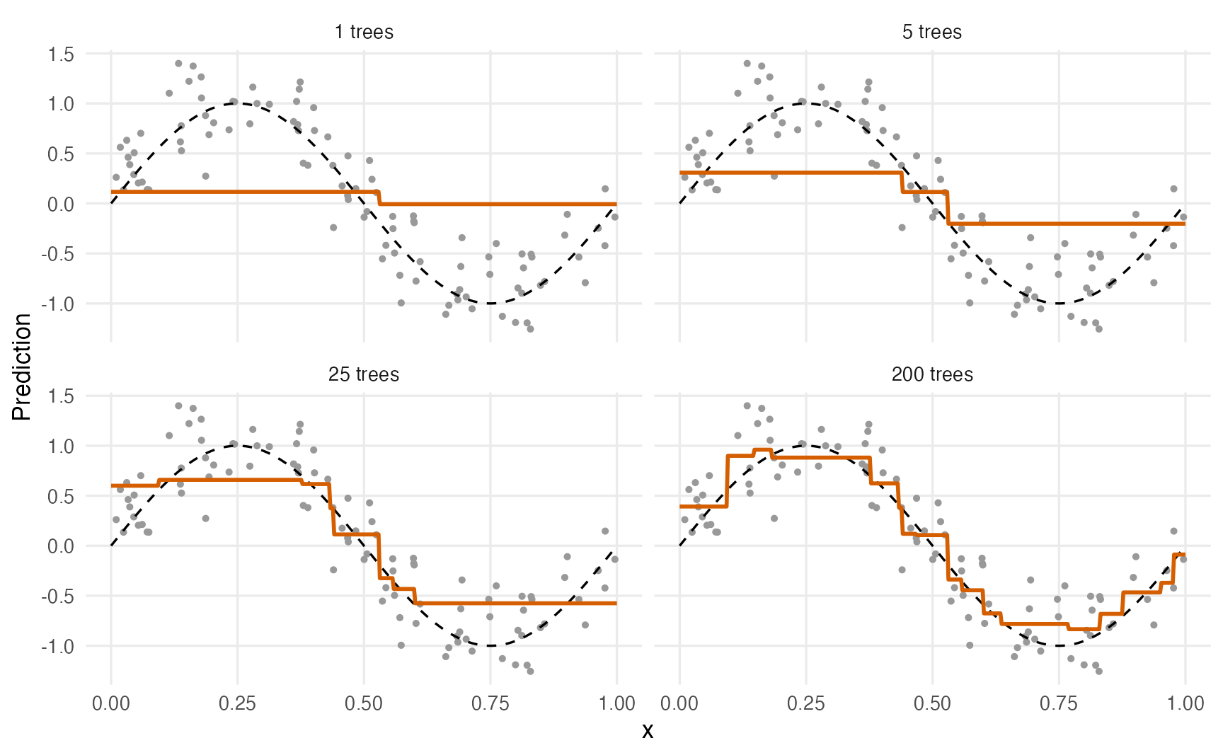

Figure 1: Boosted stumps (learning rate 0.1) after 1, 5, 25 and 200 trees. Grey points: training data; dashed line: the true curve.

How to read this output

After 1 tree, the model is the overall mean plus one-tenth of the first stump: almost flat. With a learning rate of 0.1 each tree moves the prediction only a little.
After 5 and 25 trees, the step function starts to follow the wave: each new stump has been placed where the previous model was most wrong.
After 200 trees, the prediction is a staircase with many small steps that tracks the true curve closely. Every step comes from a stump; the sum of many crude pieces is a flexible function.

3. Learning rate, number of trees and early stopping

Two hyperparameters work together:

the learning rate $\nu$ (also called shrinkage or eta): how much of each new tree we add;
the number of trees $M$.

With a large learning rate, each tree makes a big correction and the model fits the training data quickly — but also starts fitting the noise quickly. With a small learning rate, many more trees are needed, but the path is smoother. Let us record the error after every tree for four learning rates:

rmse <- function(obs, pred) sqrt(mean((obs - pred)^2))
error_path <- function(model, x, y) {
  pred <- rep(model$f0, length(x))
  err <- numeric(length(model$stumps))
  for (m in seq_along(model$stumps)) {
    pred <- pred + model$learn_rate * predict_stump(model$stumps[[m]], x)
    err[m] <- rmse(y, pred)
  }
  err
}

paths <- do.call(rbind, lapply(c(1, 0.3, 0.1, 0.03), \(lr) {
  mod <- boost_stumps(train$x, train$y, n_trees = 500, learn_rate = lr)
  data.frame(learn_rate = lr, tree = 1:500,
             train = error_path(mod, train$x, train$y),
             valid = error_path(mod, valid$x, valid$y))
}))

paths |>
  tidyr::pivot_longer(c(train, valid), names_to = "data",
                      values_to = "rmse") |>
  ggplot(aes(tree, rmse, colour = factor(learn_rate), linetype = data)) +
  geom_line(linewidth = 0.8) +
  geom_hline(yintercept = 0.3, linetype = "dashed") +
  scale_x_log10() +
  scale_linetype_manual(values = c(train = "dotted", valid = "solid")) +
  coord_cartesian(ylim = c(0, 0.8)) +
  labs(x = "Number of trees (log scale)", y = "RMSE",
       colour = "Learning rate", linetype = NULL)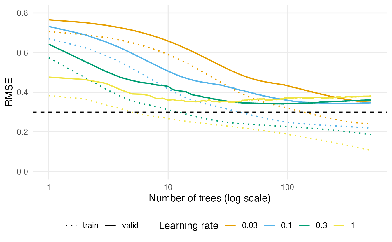

Figure 2: Training (dotted) and validation (solid) RMSE after each tree, for four learning rates. The dashed horizontal line is the noise level 0.3.

best_by_rate <- do.call(rbind, lapply(split(paths, paths$learn_rate), \(d) {
  data.frame(learn_rate = d$learn_rate[1],
             best_trees = which.min(d$valid),
             best_valid = min(d$valid),
             valid_500 = d$valid[500],
             train_500 = d$train[500])
}))
best_by_rate

#>      learn_rate best_trees best_valid valid_500 train_500
#> 0.03       0.03        500     0.3490    0.3490    0.2394
#> 0.1        0.10        295     0.3431    0.3471    0.2186
#> 0.3        0.30         92     0.3410    0.3612    0.1860
#> 1          1.00         33     0.3497    0.3810    0.1063

How to read this output

These curves are learning curves: error as a function of how long the model has been trained.

The training error (dotted) only goes down. With learning rate 1 it reaches 0.11 after 500 trees — far below the noise level of 0.3, which means the model is memorising noise.
The validation error (solid) first goes down, reaches a minimum and then slowly rises: more trees eventually mean overfitting. Unlike a random forest, a boosted model can overfit by adding trees.
The smaller the learning rate, the later the minimum: 33 trees for learning rate 1, 295 for 0.1. With 0.03, 500 trees are not even enough to reach it.
The best validation errors (best_valid) are similar across learning rates; the large rate 1 does slightly worse (0.35 against 0.341 for the best rate), because each of its steps is too coarse. A common practical rule: use a small learning rate (0.01–0.1) and enough trees, and let the data choose the number of trees.

Early stopping

Instead of fixing the number of trees in advance, we can keep adding trees and stop when the validation error has not improved for a given number of rounds (the patience). The model keeps the trees up to the best round.

early_stop <- function(valid_error, patience) {
  best <- 1
  for (m in seq_along(valid_error)) {
    if (valid_error[m] < valid_error[best]) best <- m
    if (m - best >= patience) break             # no improvement for a while
  }
  c(best = best, stopped_at = m)
}
early_stop(paths$valid[paths$learn_rate == 0.1], patience = 20)

#>       best stopped_at 
#>        295        315

With learning rate 0.1 and a patience of 20 rounds, training would stop after 315 trees and keep the first 295. Early stopping saves computing time and acts as a regulariser. Note that the validation data are now used to make a decision: they are part of the model-building process, and the final performance must still be measured on separate test data.

Tree depth

We used stumps (depth 1). Deeper trees capture interactions: a stump splits on one variable at a time, so a sum of stumps is an additive model, $f(x) = f_1(x_1) + f_2(x_2) + \dots$. A depth-2 tree can represent “the effect of age depends on sex”; depth $d$ allows interactions among up to $d$ variables. Boosted trees are usually shallow (depth 1–8): deep trees would make each step too big and fit noise. With one predictor, as here, depth only changes how many steps each tree adds.

4. Why “gradient” boosting?

So far we fitted each tree to the ordinary residuals $y_i - \hat f(x_i)$. That is right for squared-error loss, but for a 0/1 outcome (did the passenger survive?) the model predicts a log-odds $F(x)$, and $y - F$ makes no sense. Gradient boosting generalises the idea.

Let $L(y, F)$ be the loss — how bad a prediction $F$ is when the truth is $y$. For each observation, ask: in which direction should I move the current prediction $F_i$ to reduce the loss fastest? The answer is the negative gradient (negative derivative) of the loss with respect to the prediction. These numbers are the pseudo-residuals:

\[ r_{i} = -\left.\frac{\partial L(y_i, F)}{\partial F}\right|_{F = \hat F_{m-1}(x_i)} . \]

Each new tree is fitted to the pseudo-residuals, so boosting is gradient descent in the space of functions: every tree is a small step downhill.

Loss	$L(y, F)$	Pseudo-residual $-\partial L / \partial F$
Squared error ($y$ numeric)	$\tfrac12 (y - F)^2$	$y - F$ — the ordinary residual
Log-loss ($y \in \{0,1\}$, $p = 1/(1+e^{-F})$)	$-[y \log p + (1-y)\log(1-p)]$	$y - p$ — observed minus predicted probability

(The old version of this lesson wrote the pseudo-residual as minus the loss itself, $-L(y_i, F)$, forgetting the derivative: that quantity is always negative and does not point in a useful direction.)

We can check the log-loss row numerically, approximating the derivative with a small finite difference:

log_loss <- function(y, f) {
  p <- plogis(f)                                 # log-odds -> probability
  -(y * log(p) + (1 - y) * log(1 - p))
}
y <- c(1, 0, 1)
f <- c(-2, 0, 1.5)                               # current log-odds
h <- 1e-6
numeric_grad <- (log_loss(y, f + h) - log_loss(y, f - h)) / (2 * h)
cbind(minus_gradient = -numeric_grad, y_minus_p = y - plogis(f))

#>      minus_gradient y_minus_p
#> [1,]         0.8808    0.8808
#> [2,]        -0.5000   -0.5000
#> [3,]         0.1824    0.1824

The two columns agree. For the first passenger (survived, but predicted log-odds −2, i.e. $p \approx$ 0.12) the pseudo-residual is large and positive: the next tree will push that prediction up.

Going deeper: the algorithm and what XGBoost adds

Gradient boosting (Friedman, 2001) with loss $L$, $M$ trees and learning rate $\nu$:

$\hat F_0(x) = \arg\min_c \sum_i L(y_i, c)$ (the mean for squared error, the log-odds of the overall proportion for log-loss).
For $m = 1, \dots, M$:
1. $r_{im} = -\partial L(y_i, F)/\partial F$ at $F = \hat F_{m-1}(x_i)$;
2. fit a regression tree with $J$ leaves to $(x_i, r_{im})$, giving regions $R_{jm}$;
3. in each leaf choose $\gamma_{jm} = \arg\min_\gamma \sum_{x_i \in R_{jm}} L(y_i, \hat F_{m-1}(x_i) + \gamma)$;
4. $\hat F_m(x) = \hat F_{m-1}(x) + \nu \sum_j \gamma_{jm} \mathbf 1(x \in R_{jm})$.

For squared error, step (c) gives the leaf mean of the residuals — exactly our fit_stump().

XGBoost (Chen & Guestrin, 2016) uses a second-order (Newton) approximation of the loss, with gradients $g_i$ and second derivatives $h_i$ (for log-loss, $h_i = p_i(1 - p_i)$), and adds a penalty on each tree, \[ \Omega(T) = \gamma\, J + \tfrac12 \lambda \sum_{j=1}^J w_j^2 \;(+\, \alpha \textstyle\sum_j |w_j|), \] where $w_j$ are the leaf values. The optimal leaf value is $w_j = -\sum_{i \in j} g_i / (\sum_{i \in j} h_i + \lambda)$, and a split is made only if it reduces the penalised loss by more than $\gamma$ (loss_reduction in tidymodels). Row subsampling (sample_size) and column subsampling (mtry) add randomness, as in a random forest, which usually reduces variance further (stochastic gradient boosting).

5. XGBoost hyperparameters

The tidymodels function boost_tree() uses the same argument names for every engine. With set_engine("xgboost") they map to XGBoost parameters as follows:

`boost_tree()` argument	XGBoost name	What it controls	Typical range
`trees`	`nrounds`	Maximum number of trees $M$	100 – 2000 (with early stopping)
`learn_rate`	`eta`	Shrinkage $\nu$ of each tree	0.01 – 0.3
`tree_depth`	`max_depth`	Depth of each tree (interaction order)	1 – 8
`min_n`	`min_child_weight`	Minimum (Hessian-weighted) size of a leaf	1 – 40
`loss_reduction`	`gamma`	Minimum loss reduction needed to split ($\gamma$)	0 – 10
`sample_size`	`subsample`	Fraction of rows used for each tree	0.5 – 1
`mtry`	`colsample_bynode`	Predictors considered at each split	a few to all
`stop_iter`	`early_stopping_rounds`	Patience for early stopping	10 – 50

Other XGBoost parameters can be passed as engine arguments, e.g. set_engine("xgboost", lambda = 1, alpha = 0) for the L2 and L1 penalties on leaf values, scale_pos_weight to up-weight a rare positive class, or device = "cuda" to train on an NVIDIA GPU (the old tree_method = "gpu_hist" is deprecated).

6. Boosting the Titanic

We use the same Titanic preparation as in the ML workflow lesson:

titanic <- readr::read_csv(data_path("titanic_data.csv"),
                           na = c("", "NA", "?"), show_col_types = FALSE) |>
  select(survived, pclass, sex, age, sibsp, parch, fare, embarked) |>
  mutate(
    survived = factor(survived, levels = c(1, 0), labels = c("yes", "no")),
    pclass   = factor(pclass, levels = 1:3, labels = c("1st", "2nd", "3rd")),
    sex      = factor(sex),
    embarked = factor(embarked)
  )

set.seed(2026)
titanic_split <- initial_split(titanic, prop = 0.75, strata = survived)
titanic_train <- training(titanic_split)
titanic_test  <- testing(titanic_split)
set.seed(2026)
titanic_folds <- vfold_cv(titanic_train, v = 5, strata = survived)
titanic_metrics <- metric_set(roc_auc, accuracy, sensitivity, specificity,
                              brier_class, mn_log_loss)

Recipe

XGBoost needs numeric predictors, so factors must become dummy variables. Trees are not affected by monotone transformations, so there is no need to log fare or to normalise. (XGBoost can handle missing values itself; we impute anyway, to keep the pipeline the same as for the other models.)

xgb_rec <- recipe(survived ~ ., data = titanic_train) |>
  step_impute_median(all_numeric_predictors()) |>
  step_impute_mode(all_nominal_predictors()) |>
  step_dummy(all_nominal_predictors())

Unlike the old version of this lesson, we do not include both fare and a log-transformed copy of it (for trees they carry exactly the same information), and we do not invent an indicator “age < 18” and call it an interaction: trees of depth ≥ 2 find interactions by themselves.

Model specification and tuning

xgb_spec <- boost_tree(
  trees = 1000, tree_depth = tune(), learn_rate = tune(),
  min_n = 5, loss_reduction = 0, sample_size = 0.8, mtry = 6,
  stop_iter = 20
) |>
  set_engine("xgboost", validation = 0.2) |>
  set_mode("classification")

xgb_wf <- workflow() |>
  add_recipe(xgb_rec) |>
  add_model(xgb_spec)

trees = 1000 is only an upper limit: stop_iter = 20 stops training when the log-loss on a validation set has not improved for 20 rounds.
validation = 0.2 is an engine argument: inside every fit, 20% of the (analysis) data are held out to monitor early stopping. Without it, the monitoring would be done on the training data themselves, where the loss keeps decreasing, so early stopping would hardly ever trigger.
sample_size = 0.8 uses a random 80% of the rows for each tree; mtry = 6 considers 6 of the 9 dummy-coded predictors at each split.

We tune only depth and learning rate, on a deliberately small grid:

xgb_grid <- tidyr::expand_grid(tree_depth = c(1L, 3L, 6L),
                               learn_rate = c(0.01, 0.05, 0.2))

set.seed(2026)
xgb_res <- tune_grid(xgb_wf, resamples = titanic_folds, grid = xgb_grid,
                     metrics = titanic_metrics)

autoplot(xgb_res, metric = c("roc_auc", "brier_class"))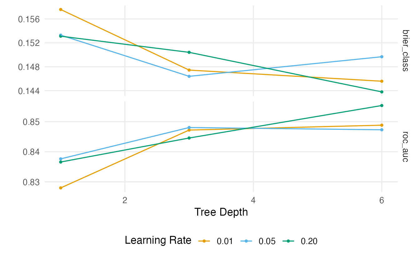

Figure 3: Cross-validated ROC AUC and Brier score of boosted trees by depth and learning rate.

show_best(xgb_res, metric = "roc_auc", n = 5)

#> # A tibble: 5 × 8
#>   tree_depth learn_rate .metric .estimator   mean     n std_err .config        
#>        <int>      <dbl> <chr>   <chr>       <dbl> <int>   <dbl> <chr>          
#> 1          6       0.2  roc_auc binary     0.8554     5 0.01177 pre0_mod9_post0
#> 2          6       0.01 roc_auc binary     0.8489     5 0.01301 pre0_mod7_post0
#> 3          3       0.05 roc_auc binary     0.8481     5 0.01626 pre0_mod5_post0
#> 4          6       0.05 roc_auc binary     0.8473     5 0.01199 pre0_mod8_post0
#> 5          3       0.01 roc_auc binary     0.8472     5 0.01300 pre0_mod4_post0

best_xgb <- select_best(xgb_res, metric = "roc_auc")
best_xgb

#> # A tibble: 1 × 3
#>   tree_depth learn_rate .config        
#>        <int>      <dbl> <chr>          
#> 1          6        0.2 pre0_mod9_post0

How to read this output

Each line in the plot is one tree depth; the x-axis is the learning rate (on a log scale). Because of early stopping, a small learning rate is compensated by more trees, so the curves are often rather flat.
The best combination is depth 6 with learning rate 0.2. Look at std_err in show_best(): several combinations are usually within one standard error of the best, so the exact choice matters little.
If depth 1 (stumps, an additive model) is as good as deeper trees, the data contain little evidence of interactions that the model can exploit.

xgb_final <- xgb_wf |>
  finalize_workflow(best_xgb) |>
  last_fit(titanic_split, metrics = titanic_metrics)
collect_metrics(xgb_final)

#> # A tibble: 6 × 4
#>   .metric     .estimator .estimate .config        
#>   <chr>       <chr>          <dbl> <chr>          
#> 1 accuracy    binary        0.8293 pre0_mod0_post0
#> 2 sensitivity binary        0.624  pre0_mod0_post0
#> 3 specificity binary        0.9557 pre0_mod0_post0
#> 4 roc_auc     binary        0.8636 pre0_mod0_post0
#> 5 brier_class binary        0.1332 pre0_mod0_post0
#> 6 mn_log_loss binary        0.4279 pre0_mod0_post0

As always, the test set is used once, for the finalised workflow. Compare these numbers with those of the logistic regression (lesson 44), the tree (lesson 45) and the forest (lesson 46). On a small data set with a few strong predictors such as this one, the differences between flexible models are usually small; a fair comparison on the same resamples is the topic of lesson 49.

collect_predictions(xgb_final) |>
  conf_mat(truth = survived, estimate = .pred_class)

#>           Truth
#> Prediction yes  no
#>        yes  78   9
#>        no   47 194

Box: faster tuning by racing

A full grid evaluates every combination on every fold. Racing (package finetune) evaluates all combinations on the first few folds and then drops those that are clearly worse, so the remaining folds are spent on promising candidates only:

library(finetune)
set.seed(2026)
xgb_race <- tune_race_anova(xgb_wf, resamples = titanic_folds,
                            grid = xgb_grid, metrics = titanic_metrics,
                            control = control_race(verbose_elim = TRUE))

The interface is the same as tune_grid(), and the result can be used with show_best() and select_best() in the same way.

7. Variable importance

xgb_final |>
  extract_fit_parsnip() |>
  plot_importance(n = 9)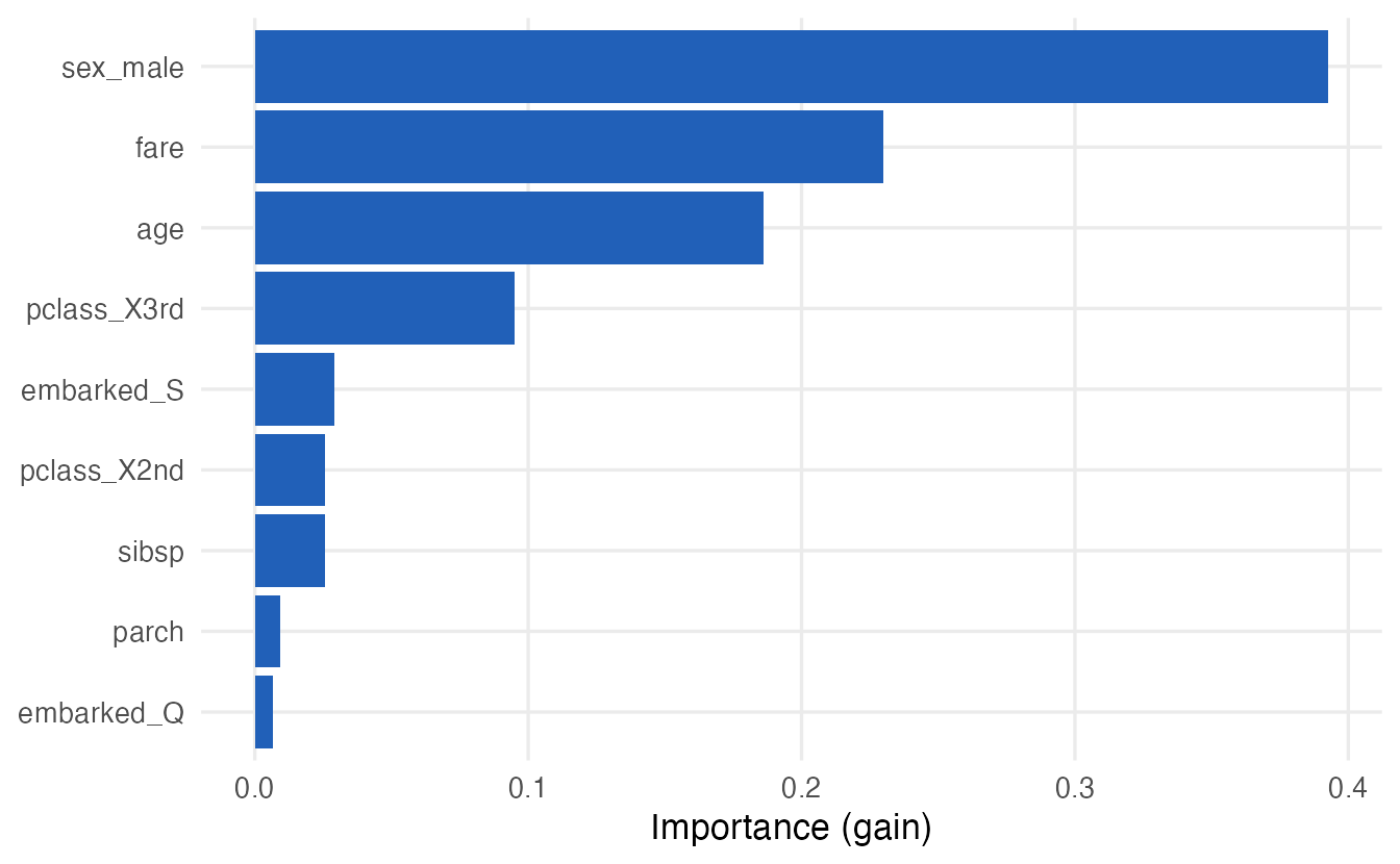

Figure 4: XGBoost gain importance of the tuned model.

plot_importance() — a small helper defined in the course file _common.R (the former vip package was archived from CRAN in 2025) — shows for XGBoost models the gain: the total improvement in the loss brought by the splits on each variable, relative to the total. It is the boosting analogue of the impurity importance of random forests, and it has the same weakness: variables with many possible split points (age, fare) can look more important than they are. The names are those of the dummy variables (sex_male, pclass_X3rd, …), because that is what the model sees. Permutation importance, computed on held-out data and on the original variables, is shown in lesson 49.

A more detailed explanation of individual predictions uses SHAP values, which split each prediction into additive contributions of the predictors. They are beyond the scope of this course; the shapviz package and Molnar’s Interpretable Machine Learning (see Further reading) are good starting points.

Box: the native xgboost R interface (version ≥ 2)

tidymodels calls the xgboost package for you. You may also meet code that uses it directly. Recent versions of the R package (2.x and 3.x) changed several names: in particular, the list of data sets monitored during training is now called evals (it used to be watchlist), and parameters are best built with xgb.params(). A minimal example, using the recipe to produce numeric matrices:

set.seed(2026)
inner <- initial_split(titanic_train, prop = 0.8, strata = survived)
rec_prep <- prep(xgb_rec, training = training(inner))
to_dmatrix <- function(df) {
  baked <- bake(rec_prep, new_data = df)
  xgb.DMatrix(data = as.matrix(select(baked, -survived)),
              label = as.integer(baked$survived == "yes"))
}
dtrain <- to_dmatrix(training(inner))
dvalid <- to_dmatrix(testing(inner))

bst <- xgb.train(
  params = xgb.params(objective = "binary:logistic", eval_metric = "logloss",
                      max_depth = 3, learning_rate = 0.05, subsample = 0.8),
  data = dtrain,
  nrounds = 1000,
  evals = list(train = dtrain, valid = dvalid),
  early_stopping_rounds = 20,
  verbose = 0
)

The label must be numeric 0/1, and the predictors a numeric matrix: here the recipe is estimated on the inner training part only, then applied to both parts.
early_stopping_rounds monitors the last data set in evals (here valid).
predict(bst, dvalid) returns predicted probabilities of the label 1 (survival).
xgb.cv() performs k-fold cross-validation with the same arguments plus nfold.

Details differ between versions of the package; check ?xgb.train and ?xgb.params for the version you have installed. In this course, tidymodels is the recommended interface.

Common pitfalls

Using too many trees without early stopping. Unlike forests, boosting overfits when $M$ grows. Use a validation set or CV to choose $M$.
Tuning the learning rate and the number of trees separately. They trade off: halving the learning rate roughly doubles the number of trees needed. Fix a small learning rate and let early stopping choose $M$, or tune them together.
Monitoring early stopping on the training data. The training loss always decreases, so training never stops. In tidymodels, set the validation engine argument.
Writing the pseudo-residual as the loss. It is the negative derivative of the loss with respect to the prediction ($y - p$ for log-loss), not the loss itself.
Reading gain importance as definitive. Like impurity importance it favours variables with many split points. Use permutation importance on held-out data for interpretation.
Using outdated xgboost code. watchlist → evals, tree_method = "gpu_hist" → device = "cuda".

8. Check your understanding

Q1. What is the main difference between how a random forest and a boosted model use their trees?

A forest grows large trees independently (in parallel) and averages them to reduce variance. Boosting grows small trees sequentially, each fitted to the pseudo-residuals of the current model, and adds them up; it mainly reduces bias, step by step.

Q2. The current model predicts $p = 0.9$ for a passenger who died ($y = 0$). What is the pseudo-residual under log-loss, and what will the next tree do?

$y - p = 0 - 0.9 = -0.9$. The next tree will tend to push this passenger’s log-odds down, towards a lower survival probability.

Q3. Why can a sum of stumps not represent an interaction between age and sex?

Each stump depends on a single variable, so a sum of stumps is a sum of one-variable functions, $f_1(\text{age}) + f_2(\text{sex}) + \dots$. An interaction means that the effect of age depends on sex, which needs at least one tree that splits on both, i.e. depth ≥ 2.

9. Exercises

★ Exercise 1 — predict the output. Without running it: what does boost_stumps(train$x, train$y, n_trees = 1, learn_rate = 1) predict, compared with a single stump fitted to y? Then check with all.equal().

Solution

Exactly the same. The model starts at $\bar y$; the first stump is fitted to $y - \bar y$, so its leaf values are the leaf means of $y$ minus $\bar y$; adding all of it (learning rate 1) gives back the leaf means of $y$.

m1 <- boost_stumps(train$x, train$y, n_trees = 1, learn_rate = 1)
all.equal(predict_boost(m1, test$x),
          predict_stump(fit_stump(train$x, train$y), test$x))   # TRUE

★★ Exercise 2 — patience. Fit 500 boosted stumps with learning rate 0.3 and compute the validation error path. Apply early_stop() with patience 5, 20 and 50. How do the chosen number of trees and the corresponding test RMSE change?

Solution

mod03 <- boost_stumps(train$x, train$y, n_trees = 500, learn_rate = 0.3)
v03 <- error_path(mod03, valid$x, valid$y)
t03 <- error_path(mod03, test$x, test$y)
sapply(c(5, 20, 50), \(p) {
  es <- early_stop(v03, p)
  c(es, test_rmse = t03[es["best"]])
})

With patience 5, training stops early at a local minimum (about 83 trees); patience 20 and 50 both find the minimum around 92 trees, at the cost of fitting more trees before stopping. The test RMSE is about 0.325 in all three cases: once the number of trees is in a reasonable range, the result is not very sensitive to the patience.

★★ Exercise 3 — debug the old lesson. The old version of this lesson wrote the pseudo-residuals as $r_{im} = -L(y_i, F_{m-1}(x_i))$, and its “hyperparameter grid search” was

param_grid <- expand.grid(max_depth = c(3, 4, 5), eta = c(0.05, 0.1, 0.15))
best_params <- param_grid[1, ]

Explain the two problems.

Solution

The pseudo-residual is the negative derivative of the loss with respect to the current prediction, $-\partial L/\partial F$, not minus the loss. Minus the log-loss is always negative and says nothing about the direction in which the prediction should move; the correct value is $y_i - p_i$. (2) The “grid search” never fits anything: it builds a grid and takes its first row. A real search fits every combination on resamples and compares their performance, e.g. with tune_grid() as in section 6.

★★★ Exercise 4 — boosting for a 0/1 outcome. Modify boost_stumps() into boost_logit() for a 0/1 outcome: start from the log-odds of the overall proportion (qlogis(mean(y01))), and fit each stump to the pseudo-residuals $y - p$, where $p$ = plogis() of the current log-odds. Test it on simulated data with x <- runif(300) and y <- rbinom(300, 1, plogis(3 * sin(2 * pi * x))), with 200 trees and learning rate 0.1. Compare the fitted probabilities with the true ones at a few values of $x$.

Solution

boost_logit <- function(x, y01, n_trees, learn_rate) {
  f0 <- qlogis(mean(y01))
  f <- rep(f0, length(y01))
  stumps <- vector("list", n_trees)
  for (m in seq_len(n_trees)) {
    r <- y01 - plogis(f)                  # negative gradient of log-loss
    stumps[[m]] <- fit_stump(x, r)
    f <- f + learn_rate * predict_stump(stumps[[m]], x)
  }
  list(f0 = f0, stumps = stumps, learn_rate = learn_rate)
}
set.seed(471)
xc <- runif(300)
yc <- rbinom(300, 1, plogis(3 * sin(2 * pi * xc)))
mc <- boost_logit(xc, yc, n_trees = 200, learn_rate = 0.1)
x0 <- c(0.1, 0.25, 0.5, 0.75, 0.9)
round(cbind(x0, fitted = plogis(predict_boost(mc, x0)),
            true = plogis(3 * sin(2 * pi * x0))), 2)

predict_boost() can be reused because it simply adds up the shrunken stumps (now on the log-odds scale). The fitted probabilities follow the true curve: high (about 0.8) for $x < 0.5$, low (about 0.16) for $x > 0.5$, though less extreme than the truth near 0.25 and 0.75 — with only 300 noisy 0/1 outcomes the model is shrunk towards the middle. Real implementations also use a Newton step for the leaf values (see Going deeper), which converges faster.

★★ Exercise 5 — tune more, carefully. Extend the Titanic grid to also tune min_n (values 2 and 20) and sample_size (0.5 and 1). How many models are fitted in total by tune_grid() with 5 folds? Run it and compare the best ROC AUC with that of section 6: is the improvement larger than its standard error?

Solution

The grid has $3 \times 3 \times 2 \times 2 = 36$ combinations, so $36 \times 5 = 180$ boosted models.

xgb_spec2 <- xgb_spec |>
  set_args(min_n = tune(), sample_size = tune())
xgb_grid2 <- tidyr::expand_grid(tree_depth = c(1L, 3L, 6L),
                                learn_rate = c(0.01, 0.05, 0.2),
                                min_n = c(2L, 20L),
                                sample_size = c(0.5, 1))
set.seed(2026)
xgb_res2 <- tune_grid(xgb_wf |> update_model(xgb_spec2),
                      resamples = titanic_folds, grid = xgb_grid2,
                      metrics = titanic_metrics)
show_best(xgb_res2, metric = "roc_auc", n = 3)
show_best(xgb_res, metric = "roc_auc", n = 1)

Typically the best AUC changes only in the third decimal, well within one standard error: on this data set, depth and learning rate (with early stopping) matter more than the other parameters. A bigger grid also increases the risk of selecting a combination that is lucky on these particular folds.

Summary

Idea / function	What it does
Boosting	Sum of small trees, each fitted to the pseudo-residuals of the current model
Pseudo-residual $-\partial L/\partial F$	$y - F$ for squared error, $y - p$ for log-loss
Learning rate $\nu$ (`learn_rate`)	Fraction of each tree added; small = slower but smoother
Number of trees (`trees`) + early stopping (`stop_iter`)	Stop when validation loss stops improving
Depth (`tree_depth`)	Order of interactions; boosting uses shallow trees
`boost_tree(...) \\|> set_engine("xgboost", validation = 0.2)`	tidymodels XGBoost specification with an early-stopping set
`tune_grid()`, `select_best()`, `last_fit()`	Tune on CV folds, finalise, evaluate once on the test set
`plot_importance()` (course helper)	Gain importance (biased like impurity importance)
`xgb.train(params = xgb.params(...), evals = ...)`	Native xgboost interface (≥ 2)

Boosting reduces bias step by step; forests reduce variance by averaging.
Boosted models can overfit by adding trees: always choose $M$ on validation data.
Small learning rate + early stopping is a robust default.
“Gradient” boosting means each tree is a step along the negative gradient of the loss.

Loss	\(L(y, F)\)	Pseudo-residual \(-\partial L / \partial F\)
Squared error (\(y\) numeric)	\(\tfrac12 (y - F)^2\)	\(y - F\) — the ordinary residual
Log-loss (\(y \in \{0,1\}\), \(p = 1/(1+e^{-F})\))	\(-[y \log p + (1-y)\log(1-p)]\)	\(y - p\) — observed minus predicted probability