Analysis of variance (ANOVA)

Comparing several means at once — one-way and two-way designs, diagnostics and transformations

Understand ANOVA as a comparison of between-group and within-group variability, fit one-way and two-way models with aov(), check residuals, handle unequal variances with Welch’s ANOVA or a transformation, and follow up with Tukey’s comparisons.

Level 3 · Inference ⏱ ~90 min Prerequisites: t-tests, Hypothesis testing

NoteLearning objectives

By the end of this lesson you will be able to:

• explain why we use ANOVA instead of many t-tests, and what the F ratio compares;
• fit a one-way ANOVA with aov() (or lm() + anova()) and report η²;
• check the assumptions with residual plots, and use Welch’s ANOVA or a transformation when variances differ;
• identify which groups differ with Tukey’s HSD;
• fit and interpret a two-way ANOVA with an interaction, using an interaction plot.

library(dplyr)
library(ggplot2)
library(readr)

1. Why not just run many t-tests?

PlantGrowth has three groups (a control and two treatments). With \(k\) groups there are \(k(k-1)/2\) pairs: 3 pairs for 3 groups, 10 pairs for 5 groups. Each t-test at \(\alpha = 0.05\) has a 5% chance of a false positive, so with many tests the chance of at least one false alarm grows (see Hypothesis testing).

A quick simulation: 5 groups of 10 observations, all drawn from the same population, and all 10 pairwise t-tests.

set.seed(2026)
any_sig <- replicate(2000, {
  y <- rnorm(50)
  g <- factor(rep(1:5, each = 10))
  p <- pairwise.t.test(y, g, p.adjust.method = "none")$p.value
  any(p < 0.05, na.rm = TRUE)
})
mean(any_sig)

#> [1] 0.292

Even though there are no differences at all, about 29% of these “studies” find at least one “significant” pair. ANOVA answers the overall question — are all the means equal? — with one test at level \(\alpha\).

2. The intuition: between versus within

PlantGrowth |>
  summarise(n = n(), mean = mean(weight), sd = sd(weight), .by = group)

#>   group  n  mean     sd
#> 1  ctrl 10 5.032 0.5831
#> 2  trt1 10 4.661 0.7937
#> 3  trt2 10 5.526 0.4426

The group means differ. ANOVA asks whether they differ more than we would expect given how much plants vary inside each group. The total variability is split into two parts:

• between groups: how far the group means are from the grand mean;
• within groups: how far each plant is from its own group mean.

grand_mean <- mean(PlantGrowth$weight)

plants <- PlantGrowth |>
  mutate(id = row_number()) |>
  mutate(group_mean = mean(weight), .by = group)

ggplot(plants, aes(id, weight, colour = group)) +
  geom_segment(aes(xend = id, y = group_mean, yend = weight), alpha = 0.6) +
  geom_point(size = 2) +
  geom_line(aes(y = group_mean), linewidth = 1.2) +
  geom_hline(yintercept = grand_mean, linetype = "dashed") +
  labs(x = "Plant", y = "Dried weight", colour = "Group")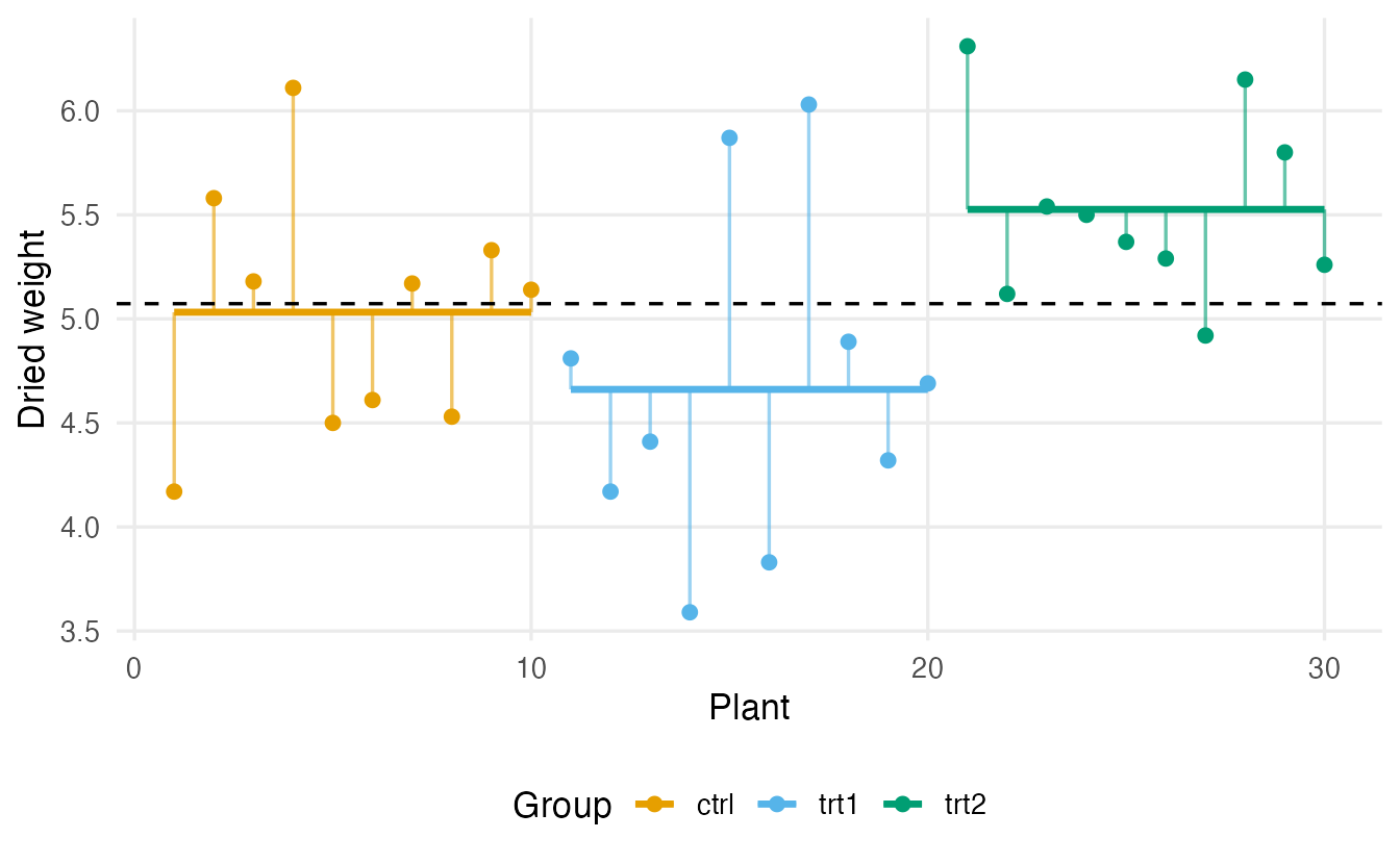

Figure 1: Decomposition of variability in PlantGrowth. Coloured horizontal lines: group means. Dashed line: grand mean. Thin vertical lines: within-group deviations of each plant from its group mean.

If the coloured lines are far from the dashed line compared with the length of the thin vertical lines, the groups really differ. The F statistic measures exactly this:

\[ F = \frac{\text{variability between groups (per degree of freedom)}}{\text{variability within groups (per degree of freedom)}} = \frac{\text{MS}_\text{between}}{\text{MS}_\text{within}} . \]

Under \(H_0\) (all population means equal) both mean squares estimate the same noise, so \(F\) is around 1. A large \(F\) means the group means are more spread out than noise alone would produce. Let us compute it by hand:

k <- 3
n <- nrow(plants)
ss_between <- sum((plants$group_mean - grand_mean)^2)
ss_within  <- sum((plants$weight - plants$group_mean)^2)

f_stat <- (ss_between / (k - 1)) / (ss_within / (n - k))
c(ss_between = ss_between, ss_within = ss_within, F = f_stat)

#> ss_between  ss_within          F 
#>      3.766     10.492      4.846

pf(f_stat, df1 = k - 1, df2 = n - k, lower.tail = FALSE)

#> [1] 0.01591

The last line is the p-value: the probability that an F distribution with 2 and 27 degrees of freedom exceeds 4.85.

NoteGoing deeper: the ANOVA identity

With \(k\) groups, \(n_j\) observations in group \(j\), group means \(\bar y_j\) and grand mean \(\bar y\):

\[ \underbrace{\sum_{j}\sum_{i}(y_{ij} - \bar y)^2}_{\text{SS}_\text{total}} = \underbrace{\sum_j n_j(\bar y_j - \bar y)^2}_{\text{SS}_\text{between}} + \underbrace{\sum_{j}\sum_{i}(y_{ij} - \bar y_j)^2}_{\text{SS}_\text{within}} . \]

Dividing by the degrees of freedom \(k-1\) and \(n-k\) gives the mean squares. If the errors are independent, normal, with equal variance, then under \(H_0\) the ratio follows an \(F_{k-1,\,n-k}\) distribution. With two groups, \(F = t^2\) for the equal-variance t-test: ANOVA generalises it.

3. One-way ANOVA in R

fit_plant <- aov(weight ~ group, data = PlantGrowth)
summary(fit_plant)

#>             Df Sum Sq Mean Sq F value Pr(>F)  
#> group        2   3.77   1.883    4.85  0.016 *
#> Residuals   27  10.49   0.389                 
#> ---
#> Signif. codes:  0 '***' 0.001 '**' 0.01 '*' 0.05 '.' 0.1 ' ' 1

TipHow to read this output

• group row: between-group variability. Df = \(k - 1\) = 2; Sum Sq = SS between; Mean Sq = Sum Sq / Df.
• Residuals row: within-group variability, with \(n - k\) = 27 degrees of freedom.
• F value = 4.85 = Mean Sq(group) / Mean Sq(residuals) — the same as our hand calculation.
• Pr(>F) = 0.0159: if all three population means were equal, an F at least this large would be rare. So at least one mean differs — but ANOVA does not say which (Section 6).

ANOVA is a linear model with a categorical predictor; lm() + anova() gives the same table and prepares you for Simple regression:

anova(lm(weight ~ group, data = PlantGrowth))

#> Analysis of Variance Table
#> 
#> Response: weight
#>           Df Sum Sq Mean Sq F value Pr(>F)  
#> group      2   3.77   1.883    4.85  0.016 *
#> Residuals 27  10.49   0.389                 
#> ---
#> Signif. codes:  0 '***' 0.001 '**' 0.01 '*' 0.05 '.' 0.1 ' ' 1

Effect size: η² (eta squared)

How much of the total variability do the groups explain?

\[ \eta^2 = \frac{\text{SS}_\text{between}}{\text{SS}_\text{total}} . \]

eta_squared <- function(fit) {
  ss <- summary(fit)[[1]][["Sum Sq"]]
  ss[1] / sum(ss)
}
eta_squared(fit_plant)

#> [1] 0.2641

The treatment group explains about 26% of the variability in plant weight. (For one-way ANOVA, η² is the \(R^2\) of the linear model.)

4. Assumptions and residual diagnostics

ANOVA assumes that the residuals (each observation minus its group mean) are

1. independent — a design question, not something a plot can check;
2. roughly normal — matters mostly for small groups;
3. of equal variance in all groups (homoscedasticity) — matters especially when group sizes differ.

Two plots check the last two:

par(mfrow = c(1, 2))
plot(fit_plant, which = 1:2)
par(mfrow = c(1, 1))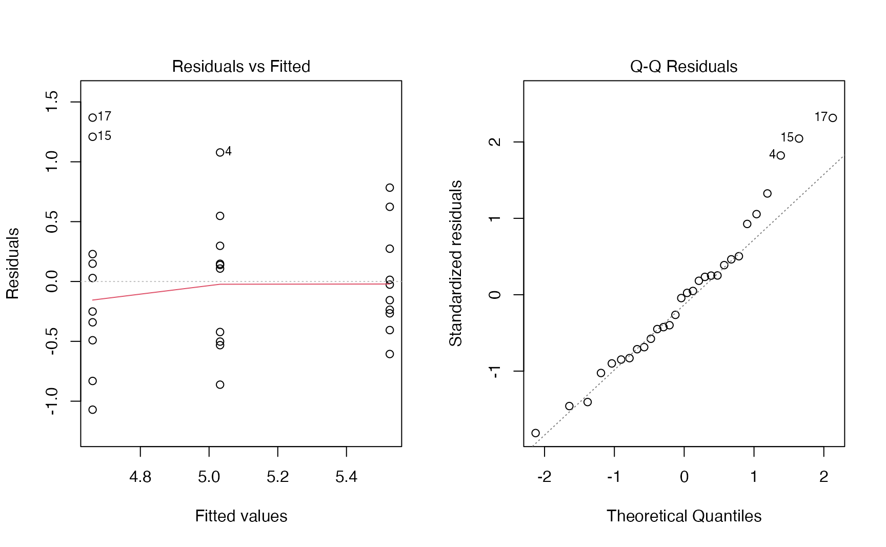

Figure 2: Residual diagnostics for the PlantGrowth ANOVA. Left: residuals against fitted values (group means). Right: normal QQ-plot of the residuals.

TipHow to read the diagnostic plots

• Residuals vs Fitted: each vertical strip is one group. We want strips of similar height, centred on 0. A funnel (spread growing with the fitted value) signals unequal variances.
• Q–Q Residuals: points close to the diagonal suggest approximately normal residuals. Look for systematic curvature or a few extreme points, not for perfection.
• Here the spreads are similar and the QQ-plot is acceptable: the assumptions look reasonable.

A formal check of equal variances is Bartlett’s test (base R), or Levene’s test, which is less sensitive to non-normality (car::leveneTest(weight ~ group, data = PlantGrowth) in the car package):

bartlett.test(weight ~ group, data = PlantGrowth)

#> 
#>  Bartlett test of homogeneity of variances
#> 
#> data:  weight by group
#> Bartlett's K-squared = 2.9, df = 2, p-value = 0.2

Treat such tests as a complement to the plots, not a gate-keeper: as for normality tests, small samples hide problems and large samples flag trivial ones.

When variances differ: Welch’s ANOVA

Just as Welch’s t-test is the safe default for two groups (t-tests), oneway.test() compares several means without assuming equal variances:

oneway.test(weight ~ group, data = PlantGrowth)

#> 
#>  One-way analysis of means (not assuming equal variances)
#> 
#> data:  weight and group
#> F = 5.2, num df = 2, denom df = 17, p-value = 0.02

Here it agrees with the classical ANOVA (p = 0.017), as expected when variances are similar. If the data are clearly non-normal with small groups, the rank-based Kruskal–Wallis test (kruskal.test(), see Non-parametric tests) is another option.

5. Which groups differ? Tukey’s HSD

Post-hoc comparisons look at all pairs while keeping the family-wise error rate at 5%. Tukey’s Honest Significant Difference is the standard choice after a one-way ANOVA:

tk_plant <- TukeyHSD(fit_plant)
tk_plant

#>   Tukey multiple comparisons of means
#>     95% family-wise confidence level
#> 
#> Fit: aov(formula = weight ~ group, data = PlantGrowth)
#> 
#> $group
#>             diff     lwr    upr  p adj
#> trt1-ctrl -0.371 -1.0622 0.3202 0.3909
#> trt2-ctrl  0.494 -0.1972 1.1852 0.1980
#> trt2-trt1  0.865  0.1738 1.5562 0.0120

plot(tk_plant, las = 1)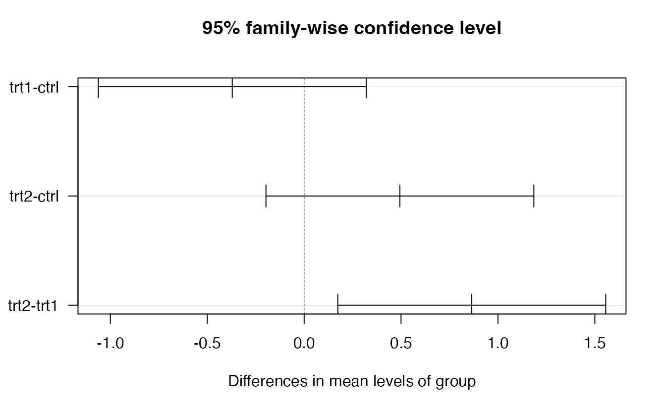

Figure 3: Tukey 95% family-wise confidence intervals for the pairwise differences in PlantGrowth. Intervals that do not cross zero indicate significant differences.

TipHow to read this output

• diff: difference between the two group means (e.g. trt2-ctrl = trt2 − ctrl).
• lwr, upr: 95% family-wise CIs: the method is built so that, in repeated experiments, all three intervals together cover the true differences 95% of the time.
• p adj: adjusted p-value. Only trt2 vs trt1 is significant (p = 0.012).
• Compare with Hypothesis testing, where a single t-test of trt2 vs ctrl gave \(p \approx 0.047\). Among three comparisons, Tukey’s adjusted p for that pair is 0.2: the evidence is weaker once we account for having looked at every pair.

6. A harder case: the poisons experiment

The poisons data (Box & Cox, 1964) come from a classic experiment: 48 animals were exposed to one of 3 poisons and given one of 4 treatments (antidotes), 4 animals per combination. The outcome is the survival time (in units of 10 hours). This is a balanced two-way design.

poisons <- read_csv(data_path("poisons.csv"),
                    col_select = c(time, poison, treat)) |>
  mutate(poison = factor(poison), treat = factor(treat))

count(poisons, poison, treat) |> head(4)

#> # A tibble: 4 × 3
#>   poison treat     n
#>   <fct>  <fct> <int>
#> 1 1      A         4
#> 2 1      B         4
#> 3 1      C         4
#> 4 1      D         4

One-way first: does the poison matter?

poisons |>
  summarise(n = n(), mean = mean(time), sd = sd(time), .by = poison)

#> # A tibble: 3 × 4
#>   poison     n   mean      sd
#>   <fct>  <int>  <dbl>   <dbl>
#> 1 1         16 0.6175 0.2094 
#> 2 2         16 0.5444 0.2894 
#> 3 3         16 0.2762 0.06228

fit_poison <- aov(time ~ poison, data = poisons)
summary(fit_poison)

#>             Df Sum Sq Mean Sq F value  Pr(>F)    
#> poison       2   1.03   0.517    11.8 7.7e-05 ***
#> Residuals   45   1.97   0.044                    
#> ---
#> Signif. codes:  0 '***' 0.001 '**' 0.01 '*' 0.05 '.' 0.1 ' ' 1

The poison clearly matters. But notice the standard deviations: poison 3, with the shortest survival times, has a much smaller spread. This is a warning sign that will become very visible in the two-way analysis.

The two-way model: main effects and interaction

With two factors we can estimate:

• the main effect of each factor (does the poison matter, averaging over treatments? does the treatment matter?);
• their interaction: does the effect of the treatment depend on the poison?

The interaction plot shows the cell means: parallel lines mean no interaction.

ggplot(poisons, aes(treat, time, colour = poison, group = poison)) +
  stat_summary(fun = mean, geom = "line", linewidth = 1) +
  stat_summary(fun = mean, geom = "point", size = 3) +
  labs(x = "Treatment", y = "Mean survival time (10 h)", colour = "Poison")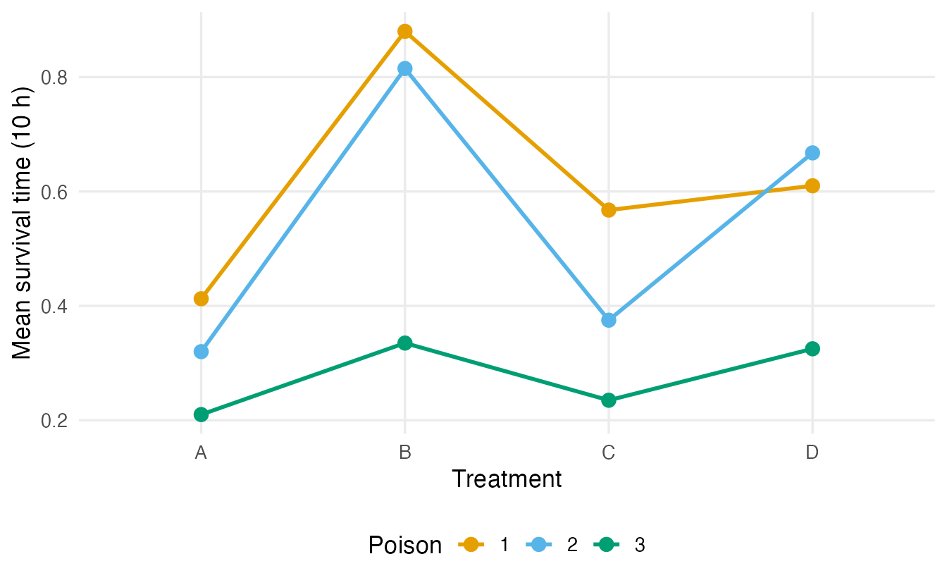

Figure 4: Interaction plot for the poisons experiment: mean survival time for each treatment, one line per poison.

fit_int <- aov(time ~ poison * treat, data = poisons)   # = poison + treat + poison:treat
summary(fit_int)

#>              Df Sum Sq Mean Sq F value  Pr(>F)    
#> poison        2  1.033   0.517   23.22 3.3e-07 ***
#> treat         3  0.921   0.307   13.81 3.8e-06 ***
#> poison:treat  6  0.250   0.042    1.87    0.11    
#> Residuals    36  0.801   0.022                    
#> ---
#> Signif. codes:  0 '***' 0.001 '**' 0.01 '*' 0.05 '.' 0.1 ' ' 1

TipHow to read this output

• poison and treat rows: the two main effects, both clearly significant.
• poison:treat: the interaction. Its p-value (0.11) gives no strong evidence that the treatment effect depends on the poison — although the plot shows lines that are not quite parallel.
• Interpret the interaction first. If it were important, a “main effect of treatment” would be an average over poisons that hides different stories.

If there is no evidence of interaction, the simpler additive model is often used:

fit_add <- aov(time ~ poison + treat, data = poisons)
summary(fit_add)

#>             Df Sum Sq Mean Sq F value  Pr(>F)    
#> poison       2  1.033   0.517    20.6 5.7e-07 ***
#> treat        3  0.921   0.307    12.3 6.7e-06 ***
#> Residuals   42  1.051   0.025                    
#> ---
#> Signif. codes:  0 '***' 0.001 '**' 0.01 '*' 0.05 '.' 0.1 ' ' 1

But first: check the residuals

par(mfrow = c(1, 2))
plot(fit_int, which = 1:2)
par(mfrow = c(1, 1))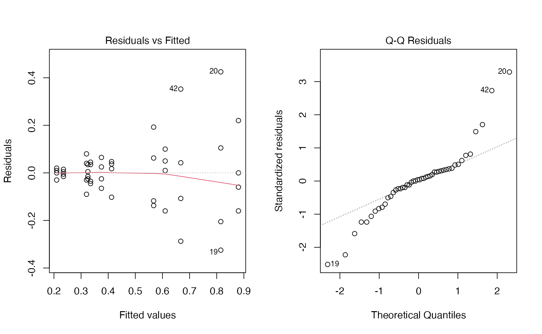

Figure 5: Residual diagnostics for the two-way model on survival time. The spread of the residuals grows with the fitted value.

The funnel in the left panel is unmistakable: cells with long average survival have far more variable residuals. The standard deviations of the 12 cells range from 0.013 to 0.336 — a factor of more than 20 — and the QQ-plot shows heavy tails. Bartlett’s test agrees:

bartlett.test(time ~ interaction(poison, treat), data = poisons)$p.value

#> [1] 4.59e-06

The equal-variance assumption is badly violated, so the F tests above are not trustworthy.

The fix: model the rate of dying

When the standard deviation grows with the mean, a transformation of the response often stabilises it. Box and Cox showed that for these data the best power transformation is close to \(y^{-1}\): the reciprocal of survival time. It has a natural meaning — \(1/\text{time}\) is the rate of dying (how fast the animal dies).

poisons <- poisons |> mutate(rate = 1 / time)

fit_rate <- aov(rate ~ poison * treat, data = poisons)
summary(fit_rate)

#>              Df Sum Sq Mean Sq F value  Pr(>F)    
#> poison        2   34.9   17.44   72.63 2.3e-13 ***
#> treat         3   20.4    6.80   28.34 1.4e-09 ***
#> poison:treat  6    1.6    0.26    1.09    0.39    
#> Residuals    36    8.6    0.24                    
#> ---
#> Signif. codes:  0 '***' 0.001 '**' 0.01 '*' 0.05 '.' 0.1 ' ' 1

par(mfrow = c(1, 2))
plot(fit_rate, which = 1:2)
par(mfrow = c(1, 1))
bartlett.test(rate ~ interaction(poison, treat), data = poisons)$p.value

#> [1] 0.5394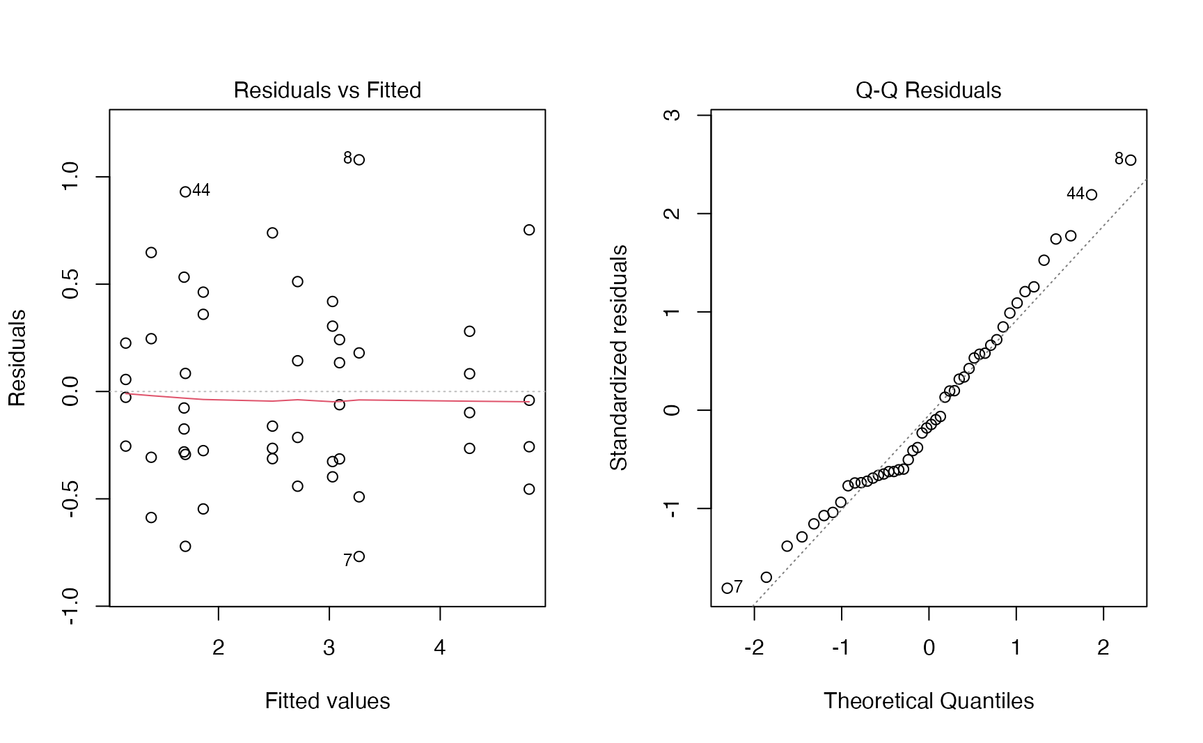

Figure 6: Residual diagnostics after the reciprocal transformation (rate of dying = 1 / time). The funnel has disappeared.

TipBefore and after the transformation

• The residual spread no longer grows with the fitted value, and the QQ-plot is much closer to the line. Bartlett’s p-value goes from 4.6e-06 to 0.54.
• On the rate scale the main effects are even clearer (F = 72.6 for poison and 28.3 for treatment), and the interaction becomes negligible (p = 0.39): the apparent non-parallel lines on the time scale were largely a by-product of the unequal spread.
• Conclusion: an additive model for the rate of dying describes these data well. Poisons and treatments act (approximately) independently on the rate.

Post-hoc comparisons on the additive model for the rate:

fit_rate_add <- aov(rate ~ poison + treat, data = poisons)
TukeyHSD(fit_rate_add, which = "poison")

#>   Tukey multiple comparisons of means
#>     95% family-wise confidence level
#> 
#> Fit: aov(formula = rate ~ poison + treat, data = poisons)
#> 
#> $poison
#>       diff     lwr    upr  p adj
#> 2-1 0.4686 0.04506 0.8922 0.0272
#> 3-1 1.9964 1.57284 2.4200 0.0000
#> 3-2 1.5278 1.10420 1.9514 0.0000

All three poisons differ; poison 3 has the highest rate of dying (it kills fastest). Remember to translate back when you report: a higher rate means a shorter survival time.

NoteGoing deeper: the Box–Cox transformation

Box and Cox (1964) proposed the family \(y^{(\lambda)} = (y^\lambda - 1)/\lambda\) (and \(\log y\) for \(\lambda = 0\)), and chose \(\lambda\) by maximum likelihood. MASS::boxcox() (the MASS package ships with R) plots the profile log-likelihood:

bc <- MASS::boxcox(time ~ poison * treat, data = poisons,
                   lambda = seq(-2, 1, by = 0.05))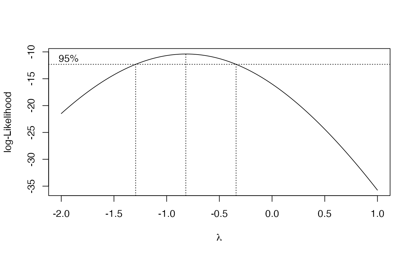

bc$x[which.max(bc$y)]

#> [1] -0.8182

The maximum is near \(\lambda =\) -0.8182, and \(\lambda = -1\) (the reciprocal) lies well inside the 95% interval shown in the plot, while \(\lambda = 1\) (no transformation) is far outside. Choosing the interpretable value \(-1\) rather than the exact optimum is standard practice. The logarithm (\(\lambda = 0\)) is a milder correction; try it in Exercise 4.

7. A second example: ToothGrowth

ToothGrowth records tooth length in 60 guinea pigs given vitamin C at three doses (0.5, 1, 2 mg/day) by two methods (supp: orange juice OJ or ascorbic acid VC), 10 animals per cell. dose is stored as a number, so we convert it to a factor — otherwise aov() would fit a straight line in dose (see Exercise 3).

tooth <- ToothGrowth |> mutate(dose = factor(dose))

fit_tooth <- aov(len ~ supp * dose, data = tooth)
summary(fit_tooth)

#>             Df Sum Sq Mean Sq F value  Pr(>F)    
#> supp         1    205     205   15.57 0.00023 ***
#> dose         2   2426    1213   92.00 < 2e-16 ***
#> supp:dose    2    108      54    4.11 0.02186 *  
#> Residuals   54    712      13                    
#> ---
#> Signif. codes:  0 '***' 0.001 '**' 0.01 '*' 0.05 '.' 0.1 ' ' 1

ggplot(tooth, aes(dose, len, colour = supp, group = supp)) +
  stat_summary(fun = mean, geom = "line", linewidth = 1) +
  stat_summary(fun = mean, geom = "point", size = 3) +
  labs(x = "Dose (mg/day)", y = "Mean tooth length", colour = "Supplement")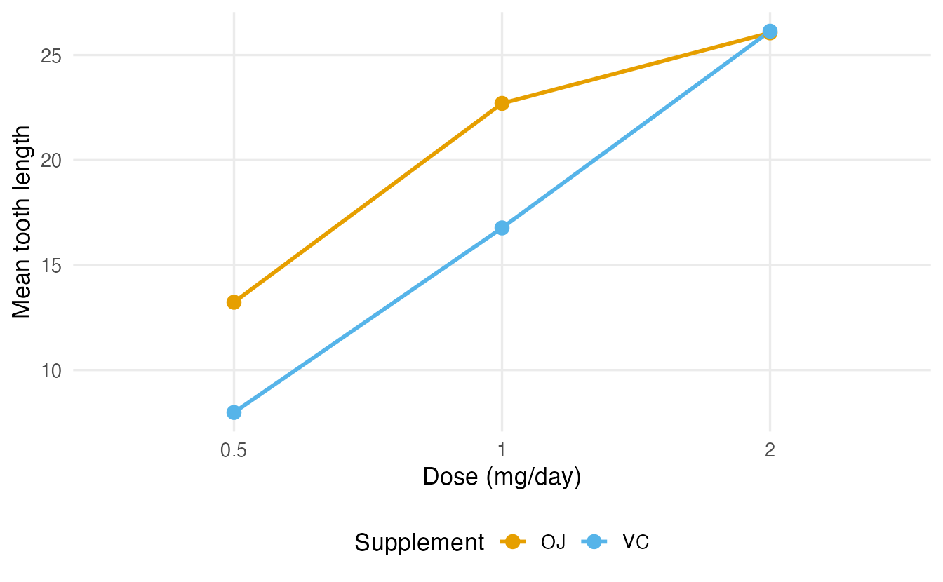

Figure 7: Interaction plot for ToothGrowth: mean tooth length by dose and supplement type.

Here the interaction is significant (p = 0.022), and the plot shows why: orange juice gives longer teeth at low and medium doses, but at 2 mg/day the two supplements give practically the same result. A single “main effect of supplement” would summarise this poorly — the honest statement is “orange juice helps more than ascorbic acid at low doses; the advantage disappears at the highest dose.”

NoteGoing deeper: unbalanced designs and types of sums of squares

In balanced designs (same \(n\) in every cell, as in poisons and ToothGrowth) the factors are uncorrelated and the ANOVA table does not depend on the order of the terms. In unbalanced designs it does. summary(aov()) and anova(lm()) use sequential (type I) sums of squares: each term is adjusted only for the terms before it.

anova(lm(mpg ~ factor(cyl) + factor(am), data = mtcars))["factor(am)", ]

#> Analysis of Variance Table
#> 
#> Response: mpg
#>            Df Sum Sq Mean Sq F value Pr(>F)  
#> factor(am)  1   36.8    36.8    3.89  0.058 .
#> ---
#> Signif. codes:  0 '***' 0.001 '**' 0.01 '*' 0.05 '.' 0.1 ' ' 1

anova(lm(mpg ~ factor(am) + factor(cyl), data = mtcars))["factor(am)", ]

#> Analysis of Variance Table
#> 
#> Response: mpg
#>            Df Sum Sq Mean Sq F value  Pr(>F)    
#> factor(am)  1    405     405    42.9 4.2e-07 ***
#> ---
#> Signif. codes:  0 '***' 0.001 '**' 0.01 '*' 0.05 '.' 0.1 ' ' 1

The sum of squares for transmission is very different depending on whether it enters first or after the number of cylinders, because the two are associated in mtcars. Alternatives:

• Type II: each main effect adjusted for the other main effects (car::Anova(fit, type = 2); for additive models drop1(fit, test = "F") gives the same tests). A sensible default when interactions are absent.
• Type III: each term adjusted for all others, including interactions (car::Anova(fit, type = 3), which requires sum-to-zero contrasts such as options(contrasts = c("contr.sum", "contr.poly"))).

With unbalanced data, state which type you used.

WarningCommon pitfalls

1. Running all pairwise t-tests instead of ANOVA + adjusted comparisons. The false-positive rate inflates quickly.
2. Forgetting to make the grouping variable a factor. With a numeric dose, aov() fits a single slope (1 df) instead of comparing groups.
3. Skipping the residual plots. A funnel shape (as in poisons) means unequal variances: use Welch’s ANOVA (oneway.test()) for one factor, or transform the response.
4. Interpreting main effects while ignoring a real interaction. Look at the interaction plot and the interaction test first.
5. Reading “significant F” as “all groups differ”. ANOVA says at least one mean differs; post-hoc tests say which.
6. Forgetting to translate back after a transformation. Higher rate = shorter time.

8. Check your understanding

NoteQ1. An ANOVA gives F ≈ 1. What does this suggest?

The group means vary about as much as you would expect from the variability within groups: no evidence that the population means differ.

NoteQ2. In a two-way ANOVA the interaction is significant. Why should you be careful with the main effects?

Because the effect of one factor depends on the level of the other. The main effect is an average over levels that may hide opposite or very different effects (as with supplement type in ToothGrowth).

NoteQ3. The residuals-vs-fitted plot shows a funnel opening to the right. Name two remedies.

Transform the response (log, reciprocal, square root, guided by Box–Cox), or — for one factor — use Welch’s ANOVA oneway.test(). A model for non-constant variance (for example a GLM, see Poisson regression) is a further option.

9. Exercises

Interactive (run in your browser)

★ Exercise 1 — one-way ANOVA and Tukey. Do the six feeds in chickwts lead to different mean weights? Fit the ANOVA, compute η², and run Tukey’s HSD.

The outcome is weight, the factor is feed; post-hoc comparisons use TukeyHSD().

fit <- aov(weight ~ feed, data = chickwts)
summary(fit)
ss <- summary(fit)[[1]][["Sum Sq"]]
ss[1] / sum(ss)          # about 0.54
TukeyHSD(fit)

The F test is highly significant and feed explains about 54% of the variability in weight. Tukey’s comparisons show, for example, that horsebean chicks are lighter than casein, meatmeal, soybean and sunflower chicks, while casein and sunflower do not differ.

★★ Exercise 2 — check the assumptions. For the InsectSprays data (insect counts for six sprays), fit a one-way ANOVA and draw the residuals-vs-fitted plot. Then run Bartlett’s test and Welch’s ANOVA. What do you conclude about the classical ANOVA?

which = 1 draws residuals vs fitted. Welch’s ANOVA is oneway.test().

plot(fit, which = 1)
bartlett.test(count ~ spray, data = InsectSprays)
oneway.test(count ~ spray, data = InsectSprays)

The residual spread clearly grows with the fitted value (a funnel), and Bartlett’s test is significant (p ≈ 0.0001): variances are unequal, as is typical for counts. Welch’s ANOVA still finds a very strong difference between sprays, so the conclusion holds, but the classical F test should not be reported uncritically. A square-root transformation or a Poisson model would be natural alternatives.

★★ Exercise 3 — debug. A student wants to compare the three doses in ToothGrowth and writes the code below. The ANOVA table shows only 1 degree of freedom for dose, not 2. Why? Fix it.

Check class(ToothGrowth$dose). How many parameters does a straight line need, and how many does a comparison of three groups need?

class(ToothGrowth$dose)   # "numeric"
fit <- aov(len ~ factor(dose), data = ToothGrowth)
summary(fit)              # Df = 2
TukeyHSD(fit)

Because dose is numeric, aov() fits a linear trend in dose (one slope, 1 df) instead of three group means. With factor(dose) the model compares the three groups (2 df). Tukey’s test then shows that all three doses differ.

Practice on your own computer

★★★ Exercise 4 — log or reciprocal? For the poisons data, fit the two-way model on log(time) and compare its diagnostics with those of the models on time and on 1 / time. Which transformation stabilises the variance best?

TipSolution

fit_log <- aov(log(time) ~ poison * treat, data = poisons)
par(mfrow = c(1, 2)); plot(fit_log, which = 1:2); par(mfrow = c(1, 1))

cells <- interaction(poisons$poison, poisons$treat)
c(time = bartlett.test(poisons$time ~ cells)$p.value,
  log  = bartlett.test(log(poisons$time) ~ cells)$p.value,
  rate = bartlett.test(poisons$rate ~ cells)$p.value)

The log helps a lot (Bartlett p ≈ 0.07 instead of ≈ 0.000005) but a mild funnel remains in the residual plot. The reciprocal removes it (p ≈ 0.54) and gives the best-looking QQ-plot, in agreement with the Box–Cox analysis (\(\lambda \approx -0.8\), closer to −1 than to 0).

★★ Exercise 5 — interpret. Write a short paragraph (3–4 sentences) reporting the ToothGrowth analysis of Section 7 for a reader without statistical training. Mention the role of dose, the interaction and what it means in practice.

TipSolution

Example: “Tooth length increased clearly with the dose of vitamin C. Orange juice produced longer teeth than pure ascorbic acid at 0.5 and 1 mg/day (on average about 5–6 units more), but at 2 mg/day the two supplements gave practically identical results. In statistical terms, the effect of the supplement type depends on the dose (a significant interaction, p ≈ 0.02). So the choice of supplement matters at low doses, but not at the highest one.”

Summary

Task	Code
One-way ANOVA	aov(y ~ g, data = df) + summary(); or anova(lm(y ~ g))
Effect size η²	SS between / SS total
Residual diagnostics	plot(fit, which = 1:2)
Equal variances	bartlett.test(y ~ g); car::leveneTest(y ~ g)
Welch ANOVA	oneway.test(y ~ g, data = df)
Rank-based alternative	kruskal.test(y ~ g, data = df)
Post-hoc comparisons	TukeyHSD(fit); plot(TukeyHSD(fit))
Two-way ANOVA	aov(y ~ A * B, data = df) (interaction); aov(y ~ A + B) (additive)
Transformation	MASS::boxcox(); e.g. 1 / time, log(y)

• ANOVA compares between-group with within-group variability: \(F\) = signal / noise.
• One overall test controls the false-positive rate; Tukey’s HSD then tells which groups differ.
• Always look at the residuals: a funnel calls for Welch’s ANOVA or a transformation.
• In two-way designs, check the interaction before interpreting main effects.
• Transformations can make a model both more valid and more interpretable (rate of dying).

NoteFurther reading

• Çetinkaya-Rundel & Hardin, Introduction to Modern Statistics (2e), chapter on comparing many means, https://openintro-ims.netlify.app
• Box, G. E. P. & Cox, D. R. (1964). An analysis of transformations. Journal of the Royal Statistical Society, Series B, 26(2), 211–252.
• R documentation: ?aov, ?TukeyHSD, ?oneway.test, ?MASS::boxcox