library(ggplot2)
library(rsample)The bootstrap
One sample, many resamples: estimating uncertainty when there is no formula
Learn the bootstrap step by step in base R: resample your data with replacement to estimate standard errors and percentile confidence intervals for a mean, a median and a correlation, see when the method fails, and meet rsample::bootstraps() and the link to bagging.
NoteLearning objectives
By the end of this lesson you will be able to:
- explain the idea of the bootstrap: resampling the sample to approximate a sampling distribution;
- implement the bootstrap in base R with
sample(x, replace = TRUE)andreplicate(); - compute a bootstrap standard error and a percentile confidence interval for a mean, a median and a correlation;
- compare a bootstrap interval with the classical t-based interval;
- recognise situations in which the bootstrap is unreliable (very small samples, extremes, dependent data).
1. The problem: we have only one sample
In the previous lesson we learned that the uncertainty of an estimate is described by its sampling distribution, and we saw it by drawing thousands of samples from a population we had built ourselves.
In real research we cannot do that. We have one sample. For the mean we are lucky: theory gives the standard error \(s/\sqrt n\) and the t-distribution gives a confidence interval. But what about
- the median of a skewed variable?
- a correlation?
- the ratio of two means, a trimmed mean, the 90th percentile, a model’s prediction error…?
For many statistics there is no simple formula, or the formula relies on assumptions (normality, large \(n\)) that we are not willing to make. The bootstrap, proposed by Bradley Efron in 1979, offers a general, computer-based answer.
2. The idea: resample the sample
If we could sample repeatedly from the population, we would. We cannot, but we have the next best thing: the sample itself, which is our best picture of the population. The bootstrap treats the sample as if it were the population and draws new samples from it:
| Real world (impossible) | Bootstrap world (possible) | |
|---|---|---|
| “Population” | the true population | our sample of size \(n\) |
| Samples | new samples of size \(n\) from the population | resamples of size \(n\) drawn with replacement from our sample |
| Statistic | \(\hat\theta\) in each new sample | \(\hat\theta^*\) in each resample |
| Variability | sampling distribution of \(\hat\theta\) | bootstrap distribution of \(\hat\theta^*\) |
The key assumption: the variability of \(\hat\theta^*\) around \(\hat\theta\) mimics the variability of \(\hat\theta\) around the true parameter \(\theta\).
Why with replacement? A resample of size \(n\) drawn without replacement from \(n\) values is just the same data shuffled. With replacement, some observations appear twice or three times and others not at all, exactly as a new random sample from the population would contain some kinds of units more often and others less.
3. The algorithm step by step
We use the ozone measurements in the built-in airquality data (New York, summer 1973). Ozone is right-skewed, so the mean and the median differ.
ozone <- airquality$Ozone[!is.na(airquality$Ozone)]
n <- length(ozone)
c(n = n, mean = mean(ozone), median = median(ozone))
#> n mean median
#> 116.00 42.13 31.50Step 1 — draw one resample of size \(n\) with replacement and compute the statistic:
set.seed(1)
resample <- sample(ozone, size = n, replace = TRUE)
mean(resample)
#> [1] 47.52Some days appear several times in the resample, others not at all:
set.seed(1)
table(table(resample_id = sample(1:n, n, replace = TRUE)))
#>
#> 1 2 3 4 5
#> 37 22 6 3 1(The output reads: so many observations were drawn once, so many twice, and so on. On average only about 63% of the original observations appear in a resample; see the “Going deeper” box in Section 7.)
Step 2 — repeat many times (B = 5,000 is plenty here) and store each statistic:
set.seed(1)
boot_means <- replicate(5000, mean(sample(ozone, replace = TRUE)))
sample(x, replace = TRUE) uses size = length(x) by default: exactly what the bootstrap needs.
Step 3 — look at the bootstrap distribution:
ci_mean <- quantile(boot_means, c(0.025, 0.975))

ggplot(data.frame(mean = boot_means), aes(mean)) +
  geom_histogram(bins = 50, fill = "#0072B2", colour = "white") +
  geom_vline(xintercept = mean(ozone), linewidth = 1) +
  geom_vline(xintercept = ci_mean, linetype = "dashed", linewidth = 0.8) +
  labs(x = "Bootstrap mean of ozone (ppb)", y = "Number of resamples")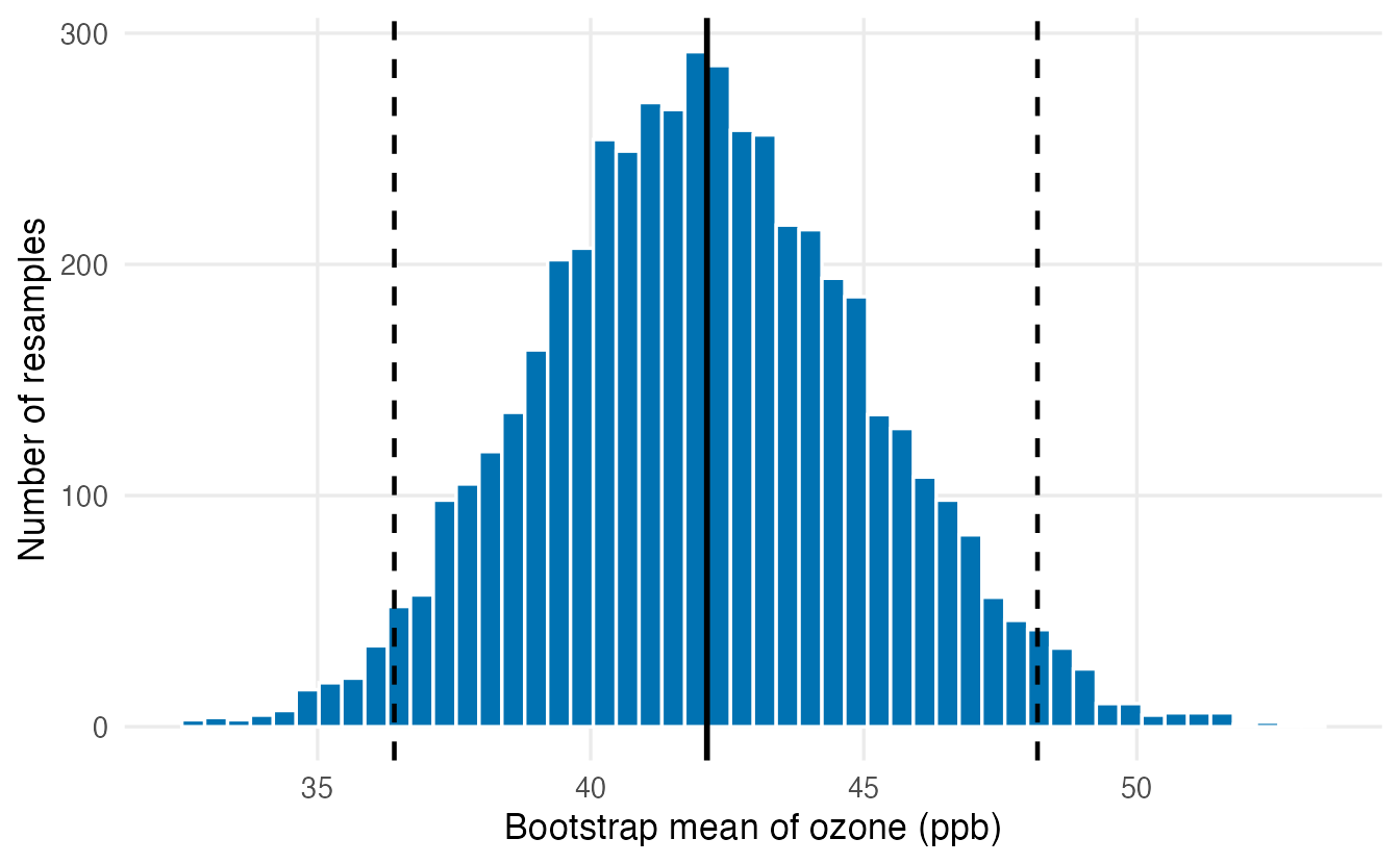
Step 4 — summarise the uncertainty.
- The bootstrap standard error is the SD of the bootstrap statistics.
- The percentile confidence interval takes the 2.5% and 97.5% quantiles of the bootstrap statistics.
sd(boot_means) # bootstrap SE#> [1] 3.026sd(ozone) / sqrt(n) # classical SE, for comparison#> [1] 3.063ci_mean # 95% percentile CI#> 2.5% 97.5%
#> 36.40 48.18
TipHow to read these results
- The bootstrap SE, 3.03, is very close to the formula \(s/\sqrt n =\) 3.06. For the mean the bootstrap simply rediscovers what theory already knew — a reassuring check.
- The 95% percentile interval runs from 36.4 to 48.2 ppb: the range of mean ozone levels compatible with the data. Confidence intervals explains exactly what “95%” means.
- Your numbers will differ slightly with a different seed; increase
Bif the second decimal matters.
Comparison with the t-based interval
t_ci <- t.test(ozone)$conf.int
rbind(t_based = t_ci[1:2], bootstrap = ci_mean)
#> 2.5% 97.5%
#> t_based 36.06 48.20
#> bootstrap 36.40 48.18The two intervals are similar. The bootstrap interval is slightly asymmetric around the mean, because the bootstrap distribution reflects the right skew of the data; the t interval is symmetric by construction. With \(n =\) 116 the CLT makes both reasonable for the mean.
NoteGoing deeper: the plug-in principle
Let \(F\) be the unknown population distribution and \(\hat F\) the empirical distribution of the sample, which puts probability \(1/n\) on each observation. Sampling with replacement from the data is sampling from \(\hat F\). The bootstrap estimates the sampling distribution of \(\hat\theta = t(X_1,\ldots,X_n)\), \(X_i \sim F\), by the distribution of \(\hat\theta^* = t(X^*_1, \ldots, X^*_n)\), \(X^*_i \sim \hat F\). Since \(\hat F \to F\) as \(n\) grows, the approximation improves with \(n\).
The percentile interval is the simplest bootstrap CI. Refinements such as the BCa (bias-corrected and accelerated) interval correct for bias and skewness and are available in the boot package (boot::boot.ci(type = "bca")). Monte Carlo error from using a finite B is a separate, controllable issue: B ≈ 1,000 is usually enough for an SE, while a few thousand are advisable for percentile CIs.
4. The real strength: statistics without a formula
The median
The median is a natural summary for skewed data, but its standard error has no simple, assumption-free formula. For the bootstrap it makes no difference: replace mean with median.
set.seed(2)
boot_medians <- replicate(5000, median(sample(ozone, replace = TRUE)))
sd(boot_medians)
#> [1] 3.639quantile(boot_medians, c(0.025, 0.975))#> 2.5% 97.5%
#> 23.00 38.01ggplot(data.frame(median = boot_medians), aes(median)) +
geom_histogram(binwidth = 0.5, fill = "#009E73") +
geom_vline(xintercept = median(ozone), linewidth = 1) +
labs(x = "Bootstrap median of ozone (ppb)", y = "Number of resamples")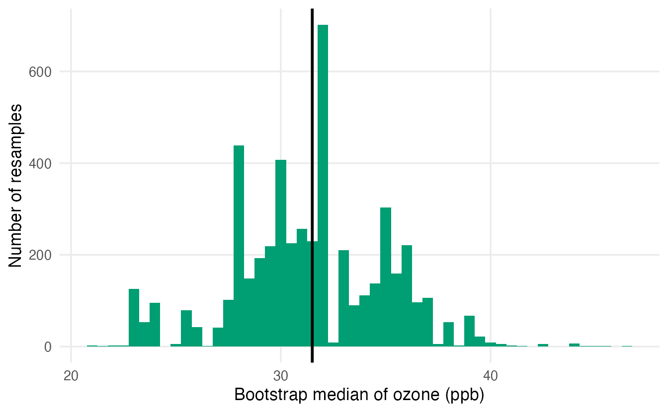
The median of ozone is 31.5 ppb with a 95% bootstrap interval from 23 to 38 ppb. The SE of the median (3.64) is larger than the SE of the mean here; the median buys robustness at the price of some precision.
A correlation
For a statistic computed from pairs of values, we must resample whole rows (units), keeping each pair together. We do this by resampling row indices. Example: the correlation between bill length and bill depth for Gentoo penguins.
gentoo <- penguins[penguins$species == "Gentoo",
                   c("bill_len", "bill_dep")]
gentoo <- gentoo[complete.cases(gentoo), ]
r_obs <- cor(gentoo$bill_len, gentoo$bill_dep)
r_obs
#> [1] 0.6434set.seed(3)
boot_cor <- replicate(5000, {
idx <- sample(nrow(gentoo), replace = TRUE) # resample rows
cor(gentoo$bill_len[idx], gentoo$bill_dep[idx])
})
sd(boot_cor)#> [1] 0.05925quantile(boot_cor, c(0.025, 0.975))#> 2.5% 97.5%
#> 0.5165 0.7445ggplot(data.frame(r = boot_cor), aes(r)) +
geom_histogram(bins = 50, fill = "#CC79A7", colour = "white") +
geom_vline(xintercept = r_obs, linewidth = 1) +
geom_vline(xintercept = quantile(boot_cor, c(0.025, 0.975)),
linetype = "dashed") +
labs(x = "Bootstrap correlation", y = "Number of resamples")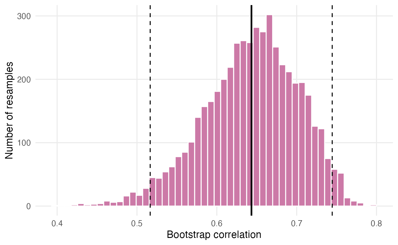
The interval from 0.52 to 0.74 excludes 0 comfortably: longer Gentoo bills tend to be deeper. Compare with the classical interval of cor.test(), which relies on a normal approximation (the Fisher transformation):
cor.test(gentoo$bill_len, gentoo$bill_dep)$conf.int#> [1] 0.5263 0.7365
#> attr(,"conf.level")
#> [1] 0.95Summary of the three intervals
data.frame(
  statistic = c("mean ozone", "median ozone", "correlation (Gentoo)"),
  estimate  = c(mean(ozone), median(ozone), r_obs),
  boot_se   = c(sd(boot_means), sd(boot_medians), sd(boot_cor)),
  lower     = c(ci_mean[1], quantile(boot_medians, 0.025),
                quantile(boot_cor, 0.025)),
  upper     = c(ci_mean[2], quantile(boot_medians, 0.975),
                quantile(boot_cor, 0.975)),
  row.names = NULL
)
#> statistic estimate boot_se lower upper
#> 1 mean ozone 42.1293 3.02629 36.4047 48.1812
#> 2 median ozone 31.5000 3.63897 23.0000 38.0125
#> 3 correlation (Gentoo) 0.6434 0.05925 0.5165 0.7445Same three lines of code each time: resample, compute, summarise. This generality is why the bootstrap is used everywhere, from medians to machine-learning performance metrics.
5. When the bootstrap fails or is risky
The bootstrap is not magic: it can only reproduce variability that is visible in the sample.
Very small samples
With 5 observations, a resample can only contain those 5 values, and the bootstrap distribution underestimates how different a new sample could be. Let us check how often a 95% interval actually contains the true mean (its coverage) when \(n = 5\) and the data are normal:
set.seed(4)
covers <- replicate(1000, {
  x <- rnorm(5)                                    # true mean is 0
  boot <- colMeans(matrix(sample(x, 5 * 1000, replace = TRUE), nrow = 5))
  pct <- quantile(boot, c(0.025, 0.975))
  tci <- t.test(x)$conf.int
  c(bootstrap = pct[[1]] < 0 & pct[[2]] > 0,
    t_based   = tci[1] < 0 & tci[2] > 0)
})
rowMeans(covers)
#> bootstrap t_based
#> 0.831 0.946(matrix(sample(...), nrow = 5) draws 1,000 resamples at once as the columns of a matrix, and colMeans() gives their means — a fast alternative to replicate().)
The “95%” percentile interval contains the true mean only about 83% of the time: it is too narrow. The t interval, which builds the extra uncertainty of small samples into the t-distribution, keeps its promise (about 95%). With small samples, prefer methods with good small-sample theory, or at least do not trust bootstrap intervals blindly.
Extremes: the maximum
The bootstrap struggles with statistics that depend on one or two extreme observations. Consider the maximum of 30 values from \(\text{Uniform}(0, 1)\); the true maximum of the population is 1.
set.seed(5)
x <- runif(30)
boot_max <- replicate(5000, max(sample(x, replace = TRUE)))
max(x)
#> [1] 0.966mean(boot_max == max(x)) # share of resamples whose max is the sample max#> [1] 0.6408max(boot_max) > max(x) # can a resample ever exceed the sample max?#> [1] FALSEAbout 64% of the resamples have exactly the same maximum as the sample, and no resample can ever go beyond it. The bootstrap distribution is a spike, nothing like the true (continuous) sampling distribution of the maximum, and it gives no hint that the true value 1 lies above every observation.
Dependent data
The basic bootstrap resamples observations independently, so it assumes the observations are independent. In a time series, today resembles yesterday; shuffling days destroys that structure and the bootstrap underestimates the uncertainty. A quick simulation with an autocorrelated series:
set.seed(6)
series <- as.numeric(arima.sim(model = list(ar = 0.7), n = 100))
naive_se <- sd(replicate(2000, mean(sample(series, replace = TRUE))))

# the true SE, from many independent series generated the same way
true_se <- sd(replicate(2000, mean(arima.sim(model = list(ar = 0.7), n = 100))))
c(naive_bootstrap = naive_se, true = true_se)
#> naive_bootstrap true
#> 0.1402 0.3337arima.sim() generates a series in which each value depends on the previous one. The naive bootstrap SE is less than half the true SE: intervals would be far too optimistic. For time series, clustered or repeated-measures data, resample blocks of consecutive observations or whole clusters (e.g. all measurements of one patient) instead of single rows.
WarningCommon pitfalls
- Resampling without replacement.
sample(x)only shuffles the data: every resample has the same mean and the “SE” is 0. Alwaysreplace = TRUE. - Resampling columns separately. For correlations, regressions or any multivariable statistic, resample rows (via indices), not each variable on its own — that destroys the relationship you are studying (Exercise 3).
- Thinking the bootstrap creates information. It does not add data; it only re-uses the sample. If the sample is small or unrepresentative, so is the bootstrap.
- Bootstrapping dependent data as if it were independent (time series, repeated measures, clusters). Resample the independent units.
- Too few resamples or no seed. Use at least 1,000 resamples (more for percentile CIs) and
set.seed()so results are reproducible.
6. A tidy alternative: rsample::bootstraps()
The tidymodels package rsample, which we will use for machine learning, provides the same resampling in a data-frame form. bootstraps(data, times = B) returns a table with one row per resample; each row holds a split object, and analysis(split) extracts the resampled data.
set.seed(3)
boots <- bootstraps(gentoo, times = 1000)
boots
#> # Bootstrap sampling
#> # A tibble: 1,000 × 2
#> splits id
#> <list> <chr>
#> 1 <split [123/48]> Bootstrap0001
#> 2 <split [123/39]> Bootstrap0002
#> 3 <split [123/44]> Bootstrap0003
#> 4 <split [123/46]> Bootstrap0004
#> 5 <split [123/47]> Bootstrap0005
#> 6 <split [123/42]> Bootstrap0006
#> 7 <split [123/36]> Bootstrap0007
#> 8 <split [123/47]> Bootstrap0008
#> 9 <split [123/43]> Bootstrap0009
#> 10 <split [123/40]> Bootstrap0010
#> # ℹ 990 more rowsboot_cor_tidy <- vapply(boots$splits, \(s) {
d <- analysis(s)
cor(d$bill_len, d$bill_dep)
}, numeric(1))
quantile(boot_cor_tidy, c(0.025, 0.975))#> 2.5% 97.5%
#> 0.5115 0.7424vapply(..., numeric(1)) applies the function to every split and checks that each result is a single number (see Iteration). The interval agrees with our base-R version up to Monte Carlo noise. The advantage of rsample is not the bootstrap itself — three lines of base R suffice — but that the same objects plug directly into the modelling tools of The ML workflow.
7. Looking ahead: bootstrap aggregating (“bagging”)
The bootstrap reappears in machine learning in a different role. A single decision tree is very sensitive to the exact data it is fitted on: change a few rows and the tree can change completely. Bagging (bootstrap aggregating) fits one tree to each bootstrap resample and averages their predictions. Averaging many noisy but different models reduces variance, just as averaging many observations reduces the SE of a mean. Random forests add one more trick (each split considers only a random subset of the variables) and are among the most widely used prediction methods; see Random forests.
NoteGoing deeper: the 63.2% rule and out-of-bag observations
The probability that a given observation is not picked in any of the \(n\) draws of a resample is \((1 - 1/n)^n \to e^{-1} \approx 0.368\). So each resample contains on average about 63.2% of the distinct original observations, and the remaining ≈ 36.8% are “out of bag”. Random forests use these left-out observations as a free test set (the out-of-bag error). A one-line check:
set.seed(7)
mean(replicate(2000, mean(!(1:100 %in% sample(100, replace = TRUE)))))
#> [1] 0.36498. Check your understanding
9. Exercises
Interactive (run in your browser)
★ Exercise 1 — bootstrap a mean. Bootstrap the mean fuel consumption mpg in mtcars with 5,000 resamples. Report the bootstrap SE and the 95% percentile interval, and compare with the t-based interval from t.test().
Resample with replace = TRUE; the SE is sd(boot); the 95% percentile interval uses the quantiles 0.025 and 0.975.
x <- mtcars$mpg
set.seed(1)
boot <- replicate(5000, mean(sample(x, replace = TRUE)))
sd(boot)                          # about 1.04
quantile(boot, c(0.025, 0.975))   # about 18.1 to 22.2
t.test(x)$conf.int                # about 17.9 to 22.3
The bootstrap interval is a little narrower than the t interval: with only 32 cars the percentile bootstrap tends to be slightly optimistic (Section 5), while the t-distribution accounts for estimating the SD.
★★ Exercise 2 — bootstrap a median. The built-in vector rivers contains the lengths (in miles) of 141 major North American rivers; it is strongly right-skewed. Compute the median and a 95% bootstrap percentile interval for it. Then draw a histogram of the bootstrap medians: why does it look lumpy?
Replace the blank with the statistic you want to bootstrap: median.
median(rivers)                                   # 425
set.seed(2)
boot_med <- replicate(5000, median(sample(rivers, replace = TRUE)))
quantile(boot_med, c(0.025, 0.975))              # roughly 380 to 490
hist(boot_med, breaks = 40, main = "Bootstrap medians", xlab = "Miles")
With \(n = 141\) (odd), the median of each resample is always one of the observed river lengths, so the bootstrap distribution can take only a limited set of values — hence the gaps and spikes. The interval is asymmetric around 425, reflecting the skew.
★★ Exercise 3 — debug the bootstrap. A student wants a bootstrap interval for the correlation between speed and dist in the built-in cars data (observed \(r \approx 0.81\)) and writes the code below. The interval is centred near 0! Find and fix the bug.
The two variables are resampled independently, so a car’s speed is paired with another car’s stopping distance. Resample row indices with idx <- sample(nrow(cars), replace = TRUE) and use cars$speed[idx] and cars$dist[idx].
set.seed(3)
boot_r <- replicate(5000, {
  idx <- sample(nrow(cars), replace = TRUE)
  cor(cars$speed[idx], cars$dist[idx])
})
quantile(boot_r, c(0.025, 0.975))   # about 0.70 to 0.88
Resampling the columns separately breaks the pairs and simulates a world with no relationship, so the “interval” was centred on 0. Resampling whole rows keeps each car’s speed and distance together.
★★★ Exercise 4 — predict the failure. Draw a sample of 50 values from \(\text{Uniform}(0, 10)\), so the true population maximum is 10. Before running the code, predict: (a) roughly what share of bootstrap maxima will equal the sample maximum? (b) Will the 95% percentile interval for the maximum contain 10?
Compare each bootstrap maximum with max(x). The chance that the largest observation is drawn at least once in 50 draws is \(1 - (1 - 1/50)^{50}\).
mean(boot_max == max(x))              # about 0.64
1 - (1 - 1/50)^50                     # theory: 0.636
quantile(boot_max, c(0.025, 0.975))   # upper limit = max(x) < 10
About 64% of resamples contain the largest observation, so their maximum equals the sample maximum. No resample can exceed max(x), so the interval never reaches the true value 10. For extremes, the bootstrap is the wrong tool.
Practice on your own computer
★★★ Exercise 5 — a difference between two groups. For Adelie penguins, estimate the difference in mean body mass between males and females with a bootstrap CI. Resample within each sex separately (why?), and compare your interval with the Welch interval of t.test(body_mass ~ sex, data = adelie).
TipSolution
adelie <- penguins[penguins$species == "Adelie" & !is.na(penguins$sex) &
                     !is.na(penguins$body_mass), ]
m <- adelie$body_mass[adelie$sex == "male"]
f <- adelie$body_mass[adelie$sex == "female"]
mean(m) - mean(f)

set.seed(5)
boot_diff <- replicate(5000, {
  mean(sample(m, replace = TRUE)) - mean(sample(f, replace = TRUE))
})
quantile(boot_diff, c(0.025, 0.975))
t.test(body_mass ~ sex, data = adelie)$conf.int   # female - male: signs flip
The males are on average about 675 g heavier, and both intervals run from roughly 575 to 775 g (the t.test() interval is for female − male, so its signs are reversed). Resampling within each group keeps the group sizes fixed, as in the original design.
Summary
| Step / function | Code | Purpose |
|---|---|---|
| One resample | sample(x, replace = TRUE) |
New sample of size \(n\) from the data |
| Resample rows | idx <- sample(nrow(df), replace = TRUE); df[idx, ] |
Keep variables paired |
| Bootstrap distribution | replicate(B, stat(sample(x, replace = TRUE))) |
Approximate sampling distribution |
| Bootstrap SE | sd(boot) |
Precision of the estimate |
| Percentile CI | quantile(boot, c(0.025, 0.975)) |
95% interval |
| Tidy resampling | rsample::bootstraps(df, times = B), analysis(split) |
Same idea in data-frame form |
- The bootstrap resamples the sample with replacement to imitate drawing new samples from the population.
- The same three steps — resample, compute, summarise — give SEs and CIs for statistics without a formula.
- For the mean, bootstrap and t-based results agree closely when \(n\) is moderate.
- It is unreliable for very small samples, extremes and dependent data; resample the independent units.
- Bootstrap + averaging = bagging, the core of random forests.