Randomness and simulation

Let R toss the coins: probability as a long-run frequency you can watch

Use sample(), set.seed() and replicate() to simulate random experiments, estimate probabilities, watch the Law of Large Numbers at work and understand expected values, basic probability rules and the base-rate fallacy.

Level 3 · Inference ⏱ ~75 min Prerequisites: Summary statistics

NoteLearning objectives

By the end of this lesson you will be able to:

• explain probability as a long-run relative frequency and see it emerge in a simulation;
• use sample() (with and without replacement, with prob =) and set.seed() to run reproducible random experiments;
• estimate a probability by simulation with replicate() and compare it with the exact answer;
• describe the Law of Large Numbers and the expected value of a random variable;
• apply the complement, addition and conditional-probability rules, and explain why a positive result from a good medical test can still be probably wrong.

library(ggplot2)

1. Why simulate?

So far we have described data: means, medians, plots. But every data set is, to some extent, the result of chance. A different group of patients, a different week of sales, a different sample of penguins — and the numbers would change.

To reason about “what could have happened instead” we need the language of probability. Probability can be taught with formulas, but there is a more direct route: let the computer repeat a random experiment thousands of times and count what happens. That is what simulation means, and R is very good at it.

Throughout this module we use one idea again and again:

If you can describe how data are generated, you can simulate them — and anything you can simulate, you can measure.

2. What is a probability?

Toss a fair coin. Will it land heads? You cannot say. Toss it 10,000 times, though, and the proportion of heads will be very close to 0.5. That stable long-run proportion is what we call the probability of heads.

• An experiment (or trial) is any process with an uncertain result: tossing a coin, rolling a die, choosing a random patient.
• An outcome is one possible result (e.g. “4”).
• An event is a set of outcomes we care about (e.g. “an even number”).
• The probability of an event, \(P(A)\), is a number between 0 (impossible) and 1 (certain): the proportion of times the event happens if we repeat the experiment many, many times.

This frequentist reading of probability is the one used by the tests and confidence intervals later in the course. And it gives us a recipe: to estimate a probability, repeat the experiment many times and compute the proportion of successes.

3. Random draws with sample()

sample(x, size) draws size elements at random from the vector x.

set.seed(2026)
sample(1:10, size = 5)                   # without replacement: no repeats

#> [1] 9 1 6 5 3

sample(1:6, size = 10, replace = TRUE)   # a die rolled 10 times

#>  [1] 4 4 5 4 2 2 3 5 6 1

sample(c("H", "T"), size = 8, replace = TRUE)

#> [1] "T" "T" "T" "T" "T" "T" "H" "H"

• Without replacement (the default) each element can be drawn at most once — like drawing cards from a deck or picking people for a survey.
• With replacement (replace = TRUE) every draw starts afresh — like rolling a die again and again.

Outcomes do not need to be equally likely. The prob = argument gives each element its own probability (they should add up to 1):

set.seed(2026)
loaded <- sample(1:6, size = 6000, replace = TRUE,
                 prob = c(0.1, 0.1, 0.1, 0.1, 0.1, 0.5))
table(loaded) / length(loaded)

#> loaded
#>       1       2       3       4       5       6 
#> 0.09817 0.09600 0.10767 0.10083 0.09717 0.50017

The six is drawn about half the time, as requested; the observed proportions are close to, but not exactly equal to, the probabilities we set. That gap is sampling variability, the hero of this module.

Reproducibility with set.seed()

Computers do not produce truly random numbers: they produce pseudo-random numbers from a deterministic algorithm that starts from a seed. Fix the seed and you get exactly the same “random” numbers every time:

set.seed(1); sample(1:100, 3)

#> [1] 68 39  1

set.seed(1); sample(1:100, 3)   # identical

#> [1] 68 39  1

sample(1:100, 3)                # the sequence continues: different numbers

#> [1] 34 87 43

Always call set.seed() at the start of a simulation you want others (or your future self) to reproduce. The value of the seed is arbitrary; what matters is that it is written down.

4. Estimating a probability by simulation

What is the probability that the sum of two dice is 7? Let us roll two dice 10,000 times.

set.seed(42)
n_sim <- 10000
die1 <- sample(1:6, n_sim, replace = TRUE)
die2 <- sample(1:6, n_sim, replace = TRUE)
total <- die1 + die2

mean(total == 7)

#> [1] 0.1679

total == 7 is a logical vector (TRUE/FALSE); mean() of a logical vector is the proportion of TRUEs. This “mean() of a condition” trick is the workhorse of every simulation in this module.

The exact answer is easy to count: 6 of the 36 equally likely pairs, \((1,6), (2,5), \ldots, (6,1)\), sum to 7, so \(P = 6/36 = 0.1667\). The simulation gave 0.1679: close, but not identical. With more repetitions it would get closer (Section 5).

The whole distribution of the sum is just as easy to estimate:

dice_df <- data.frame(total = total)
ggplot(dice_df, aes(x = factor(total))) +
  geom_bar(aes(y = after_stat(count / sum(count))), fill = "#0072B2") +
  labs(x = "Sum of two dice", y = "Proportion of rolls")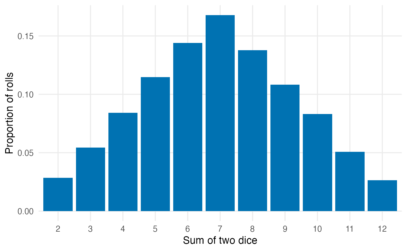

Figure 1: Simulated distribution of the sum of two dice (10,000 rolls). Sums near 7 are most likely because more pairs of faces produce them.

A general recipe with replicate()

For more complex experiments, write one run of the experiment as a block of code and let replicate() repeat it:

set.seed(42)
# Experiment: toss a coin 10 times. Do we get at least 8 heads?
at_least_8 <- replicate(10000, {
  tosses <- sample(c("H", "T"), 10, replace = TRUE)
  sum(tosses == "H") >= 8
})
mean(at_least_8)

#> [1] 0.0565

replicate(B, { ... }) evaluates the block B times and collects the last value of each run. The estimated probability of at least 8 heads in 10 tosses is about 0.056 (the exact answer, which we will compute with pbinom() in the next lesson, is 0.0547).

The birthday problem

In a class of 23 students, what is the probability that at least two share a birthday? Most people guess something small, like 5%. Simulate (ignoring leap years and assuming all 365 days are equally likely):

set.seed(1)
shared <- replicate(10000, {
  bdays <- sample(1:365, size = 23, replace = TRUE)
  any(duplicated(bdays))
})
mean(shared)

#> [1] 0.5026

About 50% — roughly a coin flip, and far more than most people guess. The surprise comes from the number of pairs: 23 students form 253 pairs, and any one of them can match.

The exact answer uses the complement (Section 7): the probability that all birthdays are different is \(\frac{365}{365}\cdot\frac{364}{365}\cdots\frac{343}{365}\).

p_shared <- function(n) 1 - prod((365 - 0:(n - 1)) / 365)
p_shared(23)

#> [1] 0.5073

set.seed(3)
class_sizes <- seq(5, 60, by = 5)
sim_est <- sapply(class_sizes, \(n) {
  mean(replicate(2000, any(duplicated(sample(365, n, replace = TRUE)))))
})
exact_df <- data.frame(n = 2:60, p = sapply(2:60, p_shared))
sim_df   <- data.frame(n = class_sizes, p = sim_est)

ggplot(exact_df, aes(n, p)) +
  geom_line(linewidth = 1, colour = "grey40") +
  geom_point(data = sim_df, colour = "#D55E00", size = 2.5) +
  geom_hline(yintercept = 0.5, linetype = "dashed") +
  labs(x = "Number of people", y = "P(at least one shared birthday)")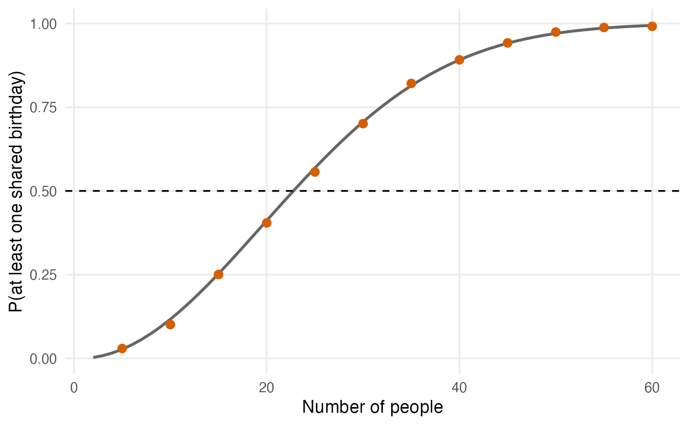

Figure 2: Probability that at least two people share a birthday: exact curve (line) and simulation estimates (points, 2,000 classes each).

Simulation and mathematics agree. This is the pattern of the whole module: when the maths is easy, simulation confirms it; when the maths is hard, simulation replaces it.

5. The Law of Large Numbers

How many repetitions are “enough”? Let us watch the proportion of heads evolve as we keep tossing a fair coin. After each toss we compute the running proportion: heads so far divided by tosses so far.

set.seed(10)
n_toss <- 5000
lln_df <- do.call(rbind, lapply(1:4, \(s) {
  heads <- sample(c(1, 0), n_toss, replace = TRUE)
  data.frame(sequence = paste("Sequence", s),
             toss = 1:n_toss,
             prop_heads = cumsum(heads) / (1:n_toss))
}))

ggplot(lln_df, aes(toss, prop_heads, colour = sequence)) +
  geom_line(linewidth = 0.7) +
  geom_hline(yintercept = 0.5, linetype = "dashed") +
  scale_x_log10() +
  labs(x = "Number of tosses (log scale)",
       y = "Running proportion of heads", colour = NULL)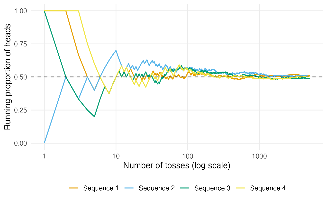

Figure 3: Running proportion of heads in four independent sequences of 5,000 fair-coin tosses (log scale on the x-axis). Early on the proportions swing wildly; in the long run they all settle near 0.5.

cumsum(heads) counts the heads accumulated after each toss; dividing by 1:n_toss turns the counts into proportions.

This is the Law of Large Numbers (LLN): as the number of independent repetitions grows, the observed proportion (or, more generally, the average) gets closer and closer to the true probability (or the true mean).

TipHow to read this plot

• After 10 tosses, proportions of 0.3 or 0.7 are perfectly normal. Small samples are noisy.
• After a few thousand tosses all four lines are within a couple of percentage points of 0.5.
• The lines settle not because the coin “compensates” for earlier streaks (it has no memory), but because early deviations are diluted by the many tosses that follow.

NoteGoing deeper: how fast does the proportion settle?

Let \(\hat p_n\) be the proportion of successes in \(n\) independent trials with success probability \(p\). The LLN says \(\hat p_n \to p\) as \(n \to \infty\). How close it is after \(n\) trials is measured by its standard deviation,

\[ \operatorname{SD}(\hat p_n) = \sqrt{\frac{p(1-p)}{n}} . \]

Quadrupling the number of trials only halves the typical error. For a fair coin, \(n = 10{,}000\) gives \(\sqrt{0.25/10000} = 0.005\), so a simulation with 10,000 repetitions estimates a probability near 0.5 to within about \(\pm 0.01\) (two standard deviations). This \(1/\sqrt n\) pattern will reappear as the standard error in Sampling distributions.

6. Random variables and expected value

A random variable is a number whose value is determined by a random experiment: the face of a die, the number of heads in 10 tosses, the body mass of a randomly chosen penguin.

• A discrete random variable takes separate, countable values (0, 1, 2, …): counts, die faces, number of defective items.
• A continuous random variable can take any value in an interval: weight, time, temperature. For a continuous variable the probability of one exact value (say, exactly 4,000.000… g) is 0; we only talk about probabilities of intervals (between 3,900 and 4,100 g). The next lesson shows how.

The expected value \(E(X)\) (or mean) of a random variable is its long-run average: the average of the values you would see if you repeated the experiment forever. For a fair die it is \((1+2+3+4+5+6)/6 = 3.5\) — a value the die can never show, but the value its average settles on:

set.seed(7)
rolls <- sample(1:6, 100000, replace = TRUE)
mean(rolls)

#> [1] 3.496

For a discrete variable with values \(x_i\) and probabilities \(p_i\), the expected value is the probability-weighted average \(E(X) = \sum_i x_i \, p_i\). Expected values help us judge bets. A game costs €1; you roll a die and win €5 if you get a six. Is it worth playing?

net <- c(4, -1)          # net gain: win (5 - 1) or lose the stake
p   <- c(1/6, 5/6)
sum(net * p)             # exact expected value

#> [1] -0.1667

set.seed(7)
games <- sample(net, 100000, replace = TRUE, prob = p)
mean(games)              # long-run average from simulation

#> [1] -0.1674

On average you lose about 0.17 euros per game. Any single game may be won, but the casino relies on the LLN.

NoteGoing deeper: expected value and variance

For a discrete random variable,

\[ E(X) = \sum_i x_i\, p_i, \qquad \operatorname{Var}(X) = E\big[(X - E X)^2\big] = \sum_i (x_i - E X)^2 p_i . \]

For a continuous variable with density \(f(x)\) the sums become integrals: \(E(X) = \int x f(x)\,dx\). The standard deviation is \(\sqrt{\operatorname{Var}(X)}\). These are the population versions of the sample mean and variance from Summary statistics; the sample versions estimate them.

7. Rules of probability, checked by simulation

Roll two dice and define three events:

• \(A\): the first die shows a 6;
• \(B\): the sum is at least 10;
• \(C\): the second die is even.

set.seed(123)
n_sim <- 100000
d1 <- sample(1:6, n_sim, replace = TRUE)
d2 <- sample(1:6, n_sim, replace = TRUE)
A <- d1 == 6
B <- d1 + d2 >= 10
C <- d2 %% 2 == 0

Complement. “Not \(A\)” happens exactly when \(A\) does not: \(P(\text{not } A) = 1 - P(A)\).

c(simulated = mean(!A), exact = 1 - 1/6)

#> simulated     exact 
#>    0.8347    0.8333

The complement rule is often the easiest way in. What is the probability of at least one six in four rolls? Directly, there are many cases (one six, two sixes, …); via the complement, it is \(1 - P(\text{no six in four rolls}) = 1 - (5/6)^4 = 0.5177\).

Addition rule. \(P(A \text{ or } B) = P(A) + P(B) - P(A \text{ and } B)\). We subtract the overlap so it is not counted twice.

c(direct  = mean(A | B),
  formula = mean(A) + mean(B) - mean(A & B))

#>  direct formula 
#>  0.2481  0.2481

Conditional probability. \(P(B \mid A)\), read “probability of \(B\) given \(A\)”, is the probability of \(B\) among the cases where \(A\) happened. In R, subset to the cases where A is TRUE and take the proportion:

c(P_B = mean(B), P_B_given_A = mean(B[A]))

#>         P_B P_B_given_A 
#>      0.1651      0.4976

Knowing that the first die is a 6 raises the probability of a sum of at least 10 from about 1/6 to about 1/2 (the second die must be 4, 5 or 6). The formula is \(P(B \mid A) = P(A \text{ and } B) / P(A)\).

Independence. Two events are independent if knowing one does not change the probability of the other: \(P(C \mid A) = P(C)\), or equivalently \(P(A \text{ and } C) = P(A)\,P(C)\).

c(P_C = mean(C), P_C_given_A = mean(C[A]))

#>         P_C P_C_given_A 
#>      0.5019      0.5002

c(P_A_and_C = mean(A & C), product = mean(A) * mean(C))

#> P_A_and_C   product 
#>   0.08268   0.08296

The two dice do not influence each other, so \(A\) and \(C\) are independent (up to simulation noise). \(A\) and \(B\) are not independent: the first die is part of the sum.

8. A two-way table: the medical test paradox

A disease affects 1% of a population. A screening test has

• sensitivity 90%: among people with the disease, 90% test positive;
• specificity 95%: among people without the disease, 95% test negative.

You test positive. What is the probability that you have the disease? Many people (including many doctors, in published surveys) answer “about 90%”. Simulate a town of 100,000 people:

set.seed(2026)
n_people <- 100000
ill <- sample(c(TRUE, FALSE), n_people, replace = TRUE,
              prob = c(0.01, 0.99))
u <- runif(n_people)           # one uniform random number per person
positive <- ifelse(ill, u < 0.90, u < 0.05)

tab <- table(Disease = ifelse(ill, "ill", "healthy"),
             Test = ifelse(positive, "positive", "negative"))
addmargins(tab)

#>          Test
#> Disease   negative positive    Sum
#>   healthy    94082     4873  98955
#>   ill          103      942   1045
#>   Sum        94185     5815 100000

runif(n) draws n numbers uniformly between 0 and 1, so u < 0.90 is TRUE with probability 0.90 — a quick way to simulate “yes with probability p”.

mean(ill[positive])     # P(ill | positive)

#> [1] 0.162

TipHow to read this table

• Read across a row to check the test: among the ill, most tested positive (sensitivity); among the healthy, most tested negative (specificity).
• Read down the positive column to answer the patient’s question. Of the 5815 positive tests, only 942 belong to ill people. The rest are false alarms from the large healthy majority: 5% of 99,000 is a lot of people.
• So \(P(\text{ill} \mid \text{positive})\) is only about 16%, even though \(P(\text{positive} \mid \text{ill})\) is 90%. These two conditional probabilities are not the same thing.

Ignoring how rare the disease is (the base rate) is called the base-rate fallacy. The same quantities — sensitivity, specificity, and the probability that a “positive” is truly positive (the positive predictive value, or precision) — will return when we evaluate classification models in Logistic regression and The ML workflow.

NoteGoing deeper: Bayes’ theorem

The exact answer follows from the definition of conditional probability:

\[ P(\text{ill} \mid +) = \frac{P(+ \mid \text{ill})\,P(\text{ill})} {P(+ \mid \text{ill})\,P(\text{ill}) + P(+ \mid \text{healthy})\,P(\text{healthy})} = \frac{0.90 \times 0.01}{0.90 \times 0.01 + 0.05 \times 0.99} \approx 0.154 . \]

The numerator counts true positives; the denominator counts all positives. This is Bayes’ theorem. Note the multiplication rule hidden inside: \(P(\text{ill and } +) = P(+ \mid \text{ill})\,P(\text{ill})\).

WarningCommon pitfalls

1. Forgetting replace = TRUE. sample(1:6, 10) fails (“cannot take a sample larger than the population”) and sample(1:6, 6) is a shuffle, not six die rolls. Dice, coins and bootstrap samples need replacement.
2. No seed, or a seed in the wrong place. Without set.seed() your numbers change every run. Put the seed in the same chunk as the simulation, just before it.
3. Expecting simulations to give the exact answer. A simulated probability is an estimate with its own error (about \(\pm 1/\sqrt{B}\) for \(B\) repetitions). Two runs with different seeds will differ slightly — that is normal.
4. The gambler’s fallacy. After five heads in a row, the next toss is still 50/50. The LLN works by dilution, not compensation.
5. Confusing \(P(A \mid B)\) with \(P(B \mid A)\). “Most ill people test positive” does not mean “most people who test positive are ill”. Always ask: among whom?
6. Multiplying probabilities of dependent events. \(P(A \text{ and } B) = P(A)\,P(B)\) only holds for independent events.

9. Check your understanding

NoteQ1. What is the difference between sample(1:52, 5) and sample(1:52, 5, replace = TRUE)?

The first deals five different cards from a deck (without replacement). The second can draw the same card more than once, as if each card were put back and the deck reshuffled before the next draw.

NoteQ2. A simulation with 100 repetitions estimates a probability as 0.31; one with 10,000 repetitions gives 0.287. Which do you trust more, and why?

The one with 10,000 repetitions. By the Law of Large Numbers the estimate gets closer to the true probability as the number of repetitions grows; its typical error is about 10 times smaller (since \(\sqrt{10000/100} = 10\)).

NoteQ3. True or false: if a die has not shown a six in the last 20 rolls, a six is now more likely.

False. Rolls are independent: the die has no memory, and the probability is still 1/6.

NoteQ4. In the medical test example, what would happen to \(P(\text{ill} \mid \text{positive})\) if the disease affected 20% of the population instead of 1%?

It would rise sharply (to about 0.82), because there would be many more true positives relative to the false positives from the healthy group. The predictive value of a test depends on the base rate, not only on its sensitivity and specificity. (Exercise 4 lets you check this.)

10. Exercises

Interactive (run in your browser)

★ Exercise 1 — two dice, two questions. Simulate 10,000 rolls of two dice and estimate (a) the probability that both dice show the same number (“a double”) and (b) the probability that the sum is at most 4. Compare with the exact answers 6/36 and 6/36.

Use replace = TRUE. A double means d1 == d2; the second event is d1 + d2 <= 4.

set.seed(1)
d1 <- sample(1:6, 10000, replace = TRUE)
d2 <- sample(1:6, 10000, replace = TRUE)
mean(d1 == d2)
mean(d1 + d2 <= 4)
6 / 36

Both estimates are close to 6/36 ≈ 0.167. (The sum is at most 4 for (1,1), (1,2), (2,1), (1,3), (2,2), (3,1): six pairs.)

★★ Exercise 2 — birthday problem. Write the experiment for a class of n people and estimate the probability of a shared birthday for n = 30 and n = 50. Then use the exact function p_shared() to find the smallest class size for which the probability exceeds 0.9.

Inside sample() the size is the class size n. which(probs > 0.9) returns all class sizes above 0.9; [1] takes the first.

sim_birthday <- function(n, B = 5000) {
  mean(replicate(B, any(duplicated(sample(365, n, replace = TRUE)))))
}
sim_birthday(30)   # about 0.71
sim_birthday(50)   # about 0.97
probs <- sapply(1:80, p_shared)
which(probs > 0.9)[1]   # 41

With 30 people a shared birthday is likely (≈ 0.71); with 41 people the probability passes 0.9.

★★ Exercise 3 — Law of Large Numbers for a die. Roll a fair die 2,000 times, compute the running mean of the rolls and plot it with a horizontal line at the expected value 3.5. Then predict: how does the plot change if you use a loaded die with prob = c(0.5, rep(0.1, 5))? Run it to check.

The running sum is cumsum(rolls). For the loaded die the expected value is sum(1:6 * c(0.5, rep(0.1, 5))).

set.seed(5)
n <- 2000
rolls <- sample(1:6, n, replace = TRUE)
running_mean <- cumsum(rolls) / (1:n)
plot(running_mean, type = "l", log = "x",
     xlab = "Number of rolls", ylab = "Running mean")
abline(h = 3.5, lty = 2)

p_loaded <- c(0.5, rep(0.1, 5))
loaded <- sample(1:6, n, replace = TRUE, prob = p_loaded)
lines(cumsum(loaded) / (1:n), col = "red")
abline(h = sum(1:6 * p_loaded), lty = 2, col = "red")   # 2.5

The fair die’s running mean settles near 3.5. The loaded die favours the 1, so its running mean settles near its own expected value, 2.5. The LLN always leads to the true mean, whatever it is.

★★★ Exercise 4 — base rates matter. Turn the medical-test simulation into a function of the prevalence and compute \(P(\text{ill} \mid \text{positive})\) for prevalences 0.001, 0.01, 0.1 and 0.2 (sensitivity 0.90, specificity 0.95). What do you conclude about screening for rare diseases?

A healthy person tests positive with probability 1 - spec. The answer is the proportion of ill people among the positives: ill[positive].

ppv_sim <- function(prev, sens = 0.90, spec = 0.95, n = 100000) {
  ill <- runif(n) < prev
  u <- runif(n)
  positive <- ifelse(ill, u < sens, u < 1 - spec)
  mean(ill[positive])
}
set.seed(1)
sapply(c(0.001, 0.01, 0.1, 0.2), ppv_sim)

The probabilities are roughly 0.02, 0.15, 0.67 and 0.82. With a rare disease almost all positives are false positives, so screening results must be confirmed with a second, more specific test.

Practice on your own computer

★★★ Exercise 5 — the Monty Hall problem. In a game show there are three doors: a car is behind one, goats behind the other two. You pick a door. The host, who knows where the car is, opens one of the other doors to reveal a goat and offers you the chance to switch. Simulate 10,000 games and estimate the probability of winning if you stay and if you switch.

TipSolution

set.seed(1)
play <- function() {
  car  <- sample(1:3, 1)
  pick <- sample(1:3, 1)
  # the host opens a goat door that is neither the pick nor the car
  goat_doors <- setdiff(1:3, c(pick, car))
  opened <- if (length(goat_doors) == 1) goat_doors else sample(goat_doors, 1)
  switched <- setdiff(1:3, c(pick, opened))
  c(stay = pick == car, switch = switched == car)
}
res <- replicate(10000, play())
rowMeans(res)

Staying wins about 1/3 of the time and switching about 2/3. Your first pick is right with probability 1/3; when it is wrong (probability 2/3), the host’s choice leaves the car behind the remaining door. Note the if guard: sample(x, 1) with a single number x would sample from 1:x, a classic R trap.

Summary

Idea / function	What it does
sample(x, size)	Draws without replacement (shuffle, deal cards)
sample(x, size, replace = TRUE, prob = p)	Draws with replacement, optionally with unequal probabilities
set.seed(n)	Makes random results reproducible
replicate(B, { ... })	Repeats one random experiment B times
mean(condition)	Proportion of TRUE = estimated probability
runif(n) < p	TRUE with probability p
cumsum(x) / seq_along(x)	Running proportion / running mean (LLN plots)
\(P(\text{not }A) = 1 - P(A)\)	Complement rule
\(P(B \mid A) = P(A \text{ and } B)/P(A)\)	Conditional probability: mean(B[A])

• A probability is a long-run relative frequency: estimate it by repeating the experiment and counting.
• The Law of Large Numbers: averages and proportions settle on their true values as repetitions grow, with error shrinking like \(1/\sqrt{n}\).
• The expected value is the long-run average of a random variable.
• \(P(A \mid B) \neq P(B \mid A)\): base rates matter, as the medical-test table shows.

NoteFurther reading

• Çetinkaya-Rundel & Hardin, Introduction to Modern Statistics (2e), https://openintro-ims.netlify.app
• Wickham, Çetinkaya-Rundel & Grolemund, R for Data Science (2e), https://r4ds.hadley.nz
• Diez, Çetinkaya-Rundel & Barr, OpenIntro Statistics (free PDF, probability chapter), https://www.openintro.org/book/os/