library(tidymodels)   # rsample, recipes, parsnip, workflows, tune,
# yardstick, dials + dplyr, ggplot2, purrr, tibbleThe machine-learning workflow
Train, validate, test — and measure honestly how well a model predicts new data
The vocabulary and logic of supervised learning: generalisation error, overfitting, the bias–variance trade-off, cross-validation, data leakage, performance metrics and baselines, followed by a complete tidymodels pipeline on the Titanic data.
NoteLearning objectives
By the end of this lesson you will be able to:
- use the vocabulary of supervised learning (features, outcome, regression vs classification) and distinguish prediction from inference;
- explain overfitting and the bias–variance trade-off with a simulation;
- estimate the performance of a model honestly with a test set and k-fold cross-validation, and recognise data leakage;
- choose and interpret metrics (RMSE, MAE, R², accuracy, sensitivity, specificity, ROC AUC, Brier score, log-loss) and compare them with a baseline;
- build a complete tidymodels pipeline: split → recipe → model → workflow → resampling → final test.
1. Why a “workflow” for prediction?
In the regression lessons we asked questions such as “how is body mass related to flipper length?” We cared about coefficients, their confidence intervals and p-values. That is inference: understanding a relationship.
Many real problems ask something different: “for a new passenger, a new patient, a new customer — what will happen?” Here we care about how accurate the predictions are on cases the model has never seen. A model can have beautiful coefficients and still predict badly; a model nobody can interpret (a forest of 1000 trees) can predict very well.
The central danger in prediction is self-deception: a flexible model can memorise the data it was trained on and look perfect — and then fail on new data. This lesson is about the habits that protect us from fooling ourselves. The next five lessons (trees, forests, boosting, SVMs, model comparison) all reuse exactly this workflow.
2. Vocabulary of supervised learning
| Term | Meaning | Titanic example |
|---|---|---|
| Outcome (target, response, \(y\)) | What we want to predict | survived (yes/no) |
| Features (predictors, inputs, \(x\)) | What we use to predict it | sex, age, pclass, fare, … |
| Observation (case, row) | One unit | One passenger |
| Supervised learning | We have examples where the outcome is known and learn a rule \(x \mapsto y\) | Passengers whose fate is recorded |
| Regression problem | Numeric outcome | Predict fare |
| Classification problem | Categorical outcome (classes) | Predict survived |
| Training | Estimating the rule from data | Fitting a logistic regression |
| Hyperparameter (tuning parameter) | A setting chosen before training, not estimated by it | Depth of a tree, number of neighbours |
Classification models usually return a probability for each class (e.g. “0.83 chance of survival”); a class prediction is then obtained by applying a threshold (by default 0.5 for two classes).
| Inference | Prediction | |
|---|---|---|
| Main question | Why / how much? | What will happen? |
| Judged by | Validity of assumptions, uncertainty of estimates | Error on new data |
| Typical tools | lm(), glm(), CIs, tests |
Resampling, test sets, metrics |
| Interpretability | Essential | Desirable, not required |
3. Overfitting and the bias–variance trade-off
A simulated world where we know the truth
Let us simulate data from a known curve, \(y = \sin(2\pi x) + \varepsilon\), with noise \(\varepsilon \sim N(0, 0.3^2)\). We train on 50 points and evaluate on 2000 new points from the same world.
As a flexible model we use k-nearest neighbours (k-NN) regression: to predict at \(x_0\), average the \(y\) of the \(k\) training points closest to \(x_0\). Small \(k\) = very flexible (with \(k = 1\) the prediction jumps from point to point); large \(k\) = very smooth (with \(k = 50\) every prediction is the overall mean).
f_true <- function(x) sin(2 * pi * x)
sim_data <- function(n, sd = 0.3) {
  x <- runif(n)
  data.frame(x = x, y = f_true(x) + rnorm(n, sd = sd))
}
knn_reg <- function(x_train, y_train, x_new, k) {
  vapply(x_new, \(x0) mean(y_train[order(abs(x_train - x0))[1:k]]),
         numeric(1))
}
rmse_vec_base <- function(obs, pred) sqrt(mean((obs - pred)^2))set.seed(44)
train_small <- sim_data(50)
test_big <- sim_data(2000)
k_values <- c(1, 2, 3, 5, 7, 10, 15, 20, 30, 40, 50)
knn_errors <- data.frame(
k = k_values,
train = sapply(k_values, \(k) rmse_vec_base(
train_small$y, knn_reg(train_small$x, train_small$y, train_small$x, k))),
test = sapply(k_values, \(k) rmse_vec_base(
test_big$y, knn_reg(train_small$x, train_small$y, test_big$x, k)))
)
knn_errors#> k train test
#> 1 1 0.0000 0.4708
#> 2 2 0.2495 0.4025
#> 3 3 0.2721 0.3951
#> 4 5 0.3082 0.3728
#> 5 7 0.3296 0.3804
#> 6 10 0.3475 0.4079
#> 7 15 0.3912 0.4308
#> 8 20 0.4527 0.4816
#> 9 30 0.5191 0.5777
#> 10 40 0.6183 0.7137
#> 11 50 0.6979 0.7912knn_errors |>
tidyr::pivot_longer(c(train, test), names_to = "data", values_to = "rmse") |>
ggplot(aes(1 / k, rmse, colour = data)) +
geom_line(linewidth = 1) +
geom_point() +
geom_hline(yintercept = 0.3, linetype = "dashed") +
scale_x_log10() +
labs(x = "Flexibility (1 / k, log scale)", y = "RMSE", colour = NULL)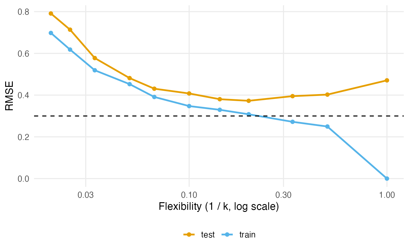
TipHow to read this output
- With \(k = 1\) the training error is 0: each training point is its own nearest neighbour, so the model “predicts” it perfectly. This is pure memorisation.
- The test error is smallest around \(k =\) 5 (RMSE 0.373), close to the irreducible noise of 0.3.
- With very large \(k\) both errors are high: the model is too rigid to follow the sine wave (underfitting).
- The gap between training and test error is a symptom of overfitting. The training error is an optimistic estimate of performance and should never be used to choose a model.
Bias and variance
Why the U shape? Imagine repeating the whole experiment many times, each time with a fresh training set of 50 points. At each \(x\) we can ask two questions:
- Bias: on average over the repetitions, is the prediction centred on the true curve?
- Variance: how much does the prediction jump around from one training set to another?
set.seed(44)
x_grid <- seq(0.05, 0.95, length.out = 40)
bv <- do.call(rbind, lapply(c(1, 3, 7, 15, 30, 50), \(k) {
  preds <- replicate(200, {
    dat <- sim_data(50)
    knn_reg(dat$x, dat$y, x_grid, k)
  })                                   # 40 x-values x 200 repetitions
  data.frame(k = k,
             bias2 = mean((rowMeans(preds) - f_true(x_grid))^2),
             variance = mean(apply(preds, 1, var)))
}))
bv$expected_mse <- bv$bias2 + bv$variance + 0.3^2
bv
#> k bias2 variance expected_mse
#> 1 1 0.0003206 0.09491 0.1852
#> 2 3 0.0003488 0.03436 0.1247
#> 3 7 0.0023675 0.02040 0.1128
#> 4 15 0.0224889 0.01538 0.1279
#> 5 30 0.1344763 0.02641 0.2509
#> 6 50 0.5402927 0.01210 0.6424Flexible models (small \(k\)) have low bias but high variance: on average they follow the curve, but each fit is noisy. Rigid models (large \(k\)) have low variance but high bias: stable, but systematically wrong. The expected test error is (approximately) the sum of the two plus the noise, and it is minimised at an intermediate complexity — here around \(k =\) 7.
NoteGoing deeper: the bias–variance decomposition
For squared-error loss, a new point \((x_0, y_0)\) with \(y_0 = f(x_0) + \varepsilon\), \(E(\varepsilon) = 0\), \(\operatorname{Var}(\varepsilon) = \sigma^2\), and a fitted model \(\hat f\) that depends on the random training set,
\[ E\big[(y_0 - \hat f(x_0))^2\big] = \underbrace{\sigma^2}_{\text{irreducible}} + \underbrace{\big(E[\hat f(x_0)] - f(x_0)\big)^2}_{\text{bias}^2} + \underbrace{\operatorname{Var}\big(\hat f(x_0)\big)}_{\text{variance}} . \]
The expectation is over both the training set and the new noise. For k-NN, \(\operatorname{Var}(\hat f(x_0)) \approx \sigma^2 / k\), which explains why variance drops as \(k\) grows. For classification with 0–1 loss the decomposition is not additive, but the same qualitative trade-off holds.
4. Honest evaluation: splitting and resampling
Train / validation / test
The fix for self-deception is simple: evaluate on data that played no role in building the model.
- Training set — used to fit models.
- Validation set — used to compare models and choose hyperparameters.
- Test set — locked away and used once, at the very end, to report the final performance.
Why three and not two? Every time you look at a data set to make a decision, it becomes part of the training process. If you try 50 models and keep the one with the best test score, that score is optimistic: you have selected it because it was lucky on those particular test rows.
k-fold cross-validation
With a few hundred observations, a single validation set is small and noisy. k-fold cross-validation (CV) re-uses the training data more efficiently:
- Split the training set into \(k\) folds of equal size (typically \(k = 5\) or \(10\)).
- For each fold: fit on the other \(k - 1\) folds, evaluate on the held-out fold.
- Average the \(k\) performance estimates (and look at their spread).
Every observation is used for evaluation exactly once and for training \(k - 1\) times. The test set is still kept aside.
Stratification
With a categorical outcome, random splits can by chance put more survivors in one fold than in another. Stratified splitting samples separately within each class, so that every split has (almost) the same class proportions as the full data. For a numeric outcome, rsample stratifies on quartiles. Use it by default: strata = outcome.
5. Data leakage
Leakage happens when information from the evaluation data sneaks into the training process. The model then looks better than it really is. Typical sources:
- Preprocessing on the full data before splitting — computing means and standard deviations for scaling, imputing missing values with the overall median, selecting “the most correlated features”, all on the whole data set.
- Features that would not be available at prediction time — e.g. using “length of hospital stay” to predict admission diagnosis.
- Duplicate or related rows in training and test (the same patient twice).
Leakage from scaling is usually small. Leakage from feature selection can be enormous. Here is a demonstration where nothing can be predicted: 100 observations, 1000 features of pure noise and a coin-flip outcome. The leaky procedure picks the 10 features most correlated with \(y\) using all the data, then runs 5-fold CV; the honest procedure repeats the selection inside each training fold.
set.seed(2026)
n <- 100
p <- 1000
x <- matrix(rnorm(n * p), nrow = n)
y <- rbinom(n, size = 1, prob = 0.5)   # outcome unrelated to x

top_k <- function(x, y, k = 10) order(-abs(cor(x, y)))[1:k]
cv_accuracy <- function(x, y, leaky, k = 10, v = 5) {
folds <- sample(rep(1:v, length.out = length(y)))
if (leaky) keep <- top_k(x, y, k) # uses ALL rows
acc <- numeric(v)
for (i in 1:v) {
tr <- folds != i
if (!leaky) keep <- top_k(x[tr, ], y[tr], k) # training fold only
d_tr <- data.frame(y = y[tr], x[tr, keep])
d_te <- data.frame(x[!tr, keep])
fit <- suppressWarnings(glm(y ~ ., data = d_tr, family = binomial))
p_hat <- predict(fit, d_te, type = "response")
acc[i] <- mean((p_hat > 0.5) == y[!tr])
}
mean(acc)
}
leaky <- replicate(20, cv_accuracy(x, y, leaky = TRUE))
honest <- replicate(20, cv_accuracy(x, y, leaky = FALSE))
c(leaky = mean(leaky), honest = mean(honest))#> leaky honest
#> 0.7445 0.4225The leaky procedure reports an accuracy of about 0.74 on data where the true accuracy of any model is 0.5. The honest procedure gives 0.42: no better than tossing a coin. (With pure noise, honest CV estimates often land somewhat below 0.5, because removing a fold slightly unbalances the classes in the training part in the opposite direction; this is a known quirk, not a skill.) The rule: every step that learns something from data — scaling, imputation, feature selection, PCA — must be estimated on the training part only and then applied to the evaluation part. In tidymodels this happens automatically when all preprocessing lives inside a recipe (section 8).
6. Metrics: what does “good” mean?
A metric turns predictions and true values into one number. Different metrics reward different things, so choose the one that matches the purpose of the model.
Regression metrics
| Metric | Formula | Rewards / punishes |
|---|---|---|
| RMSE | \(\sqrt{\frac1n\sum(y_i - \hat y_i)^2}\) | Same units as \(y\); punishes large errors heavily |
| MAE | \(\frac1n\sum \lvert y_i - \hat y_i\rvert\) | Same units; more robust to a few big errors |
| R² | \(1 - \frac{\sum(y_i-\hat y_i)^2}{\sum(y_i-\bar y)^2}\) | Proportion of variance explained relative to “predict the mean”; unitless |
pred_k7 <- knn_reg(train_small$x, train_small$y, test_big$x, k = 7)
c(rmse = sqrt(mean((test_big$y - pred_k7)^2)),
  mae  = mean(abs(test_big$y - pred_k7)),
  rsq  = 1 - sum((test_big$y - pred_k7)^2) /
             sum((test_big$y - mean(test_big$y))^2))
#> rmse mae rsq
#> 0.3804 0.3009 0.7508(yardstick’s rsq() is the squared correlation between observed and predicted values; rsq_trad() is the formula above. They coincide for a least-squares fit evaluated on its own training data, but can differ on new data — e.g. biased predictions can still be highly correlated with the truth.)
Classification metrics
Take a toy example with 200 cases, a probability for the “positive” class (1) and the default threshold 0.5:
set.seed(1)
truth <- rbinom(200, 1, 0.3)
score <- rnorm(200, mean = ifelse(truth == 1, 1, 0))
prob <- plogis(-1 + 1.2 * score)     # predicted P(class 1)
pred <- as.integer(prob > 0.5)
table(predicted = pred, truth = truth)
#> truth
#> predicted 0 1
#> 0 112 28
#> 1 26 34pos <- prob[truth == 1]
neg <- prob[truth == 0]
c(accuracy = mean(pred == truth),
sensitivity = mean(pred[truth == 1] == 1),
specificity = mean(pred[truth == 0] == 0),
roc_auc = mean(outer(pos, neg, ">")) +
0.5 * mean(outer(pos, neg, "==")),
brier = mean((prob - truth)^2),
log_loss = -mean(truth * log(prob) + (1 - truth) * log(1 - prob)))#> accuracy sensitivity specificity roc_auc brier log_loss
#> 0.7300 0.5484 0.8116 0.7835 0.1759 0.5266| Metric | What it measures | Needs | Better is |
|---|---|---|---|
| Accuracy | Share of correct class predictions | Classes (threshold) | Higher |
| Sensitivity (recall, true positive rate) | Of the true positives, how many we catch | Classes | Higher |
| Specificity (true negative rate) | Of the true negatives, how many we correctly reject | Classes | Higher |
| ROC AUC | Probability that a random positive gets a higher score than a random negative; threshold-free ranking quality | Probabilities | Higher (0.5 = random, 1 = perfect) |
| Brier score | Mean squared difference between probability and 0/1 outcome; rewards well-calibrated probabilities | Probabilities | Lower |
| Log-loss (mean negative log-likelihood) | Like Brier but punishes confident mistakes very hard | Probabilities | Lower |
The ROC curve plots sensitivity against \(1 -\) specificity for every possible threshold; AUC is the area under it. A model can have a high AUC (it ranks cases well) but poorly calibrated probabilities (e.g. it says 0.9 when the true frequency is 0.6) — Brier and log-loss detect that, AUC does not.
Class imbalance and the baseline
In the toy data, 69% of cases are 0. A “model” that always predicts 0 reaches an accuracy of 0.69 — compared with 0.73 for our model. With a rare outcome (say 2% fraud), the “always no” model has 98% accuracy and is useless.
Two habits follow:
- Always compute a baseline: predict the majority class (classification) or the training mean (regression). A model is only interesting if it clearly beats it. R² is in fact the improvement over the “predict the mean” baseline.
- With imbalanced classes, look at sensitivity/specificity, ROC AUC, Brier/log-loss, not just accuracy, and stratify your splits.
7. The Titanic data
The file data/titanic_data.csv lists the passengers of the Titanic with their fate. In this file, missing values are not coded as empty cells or NA but as a question mark "?". Let us check this with base R, reading every column as text:
raw_chr <- read.csv(data_path("titanic_data.csv"), colClasses = "character")
dim(raw_chr)
#> [1] 1309 13colSums(raw_chr == "?")#> x pclass survived name sex age sibsp parch
#> 0 0 0 0 0 263 0 0
#> ticket fare cabin embarked home.dest
#> 0 1 1014 2 564So age, fare, cabin, embarked and home.dest contain "?". If we ignored this, age would be read as text. We read the file telling read_csv() which strings mean “missing”, and keep the variables that are known at boarding time and not mostly missing:
titanic_raw <- readr::read_csv(data_path("titanic_data.csv"),
                               na = c("", "NA", "?"),
                               show_col_types = FALSE)

titanic <- titanic_raw |>
  select(survived, pclass, sex, age, sibsp, parch, fare, embarked) |>
  mutate(
    survived = factor(survived, levels = c(1, 0), labels = c("yes", "no")),
    pclass   = factor(pclass, levels = 1:3, labels = c("1st", "2nd", "3rd")),
    sex      = factor(sex),
    embarked = factor(embarked)
  )

glimpse(titanic)
#> Rows: 1,309
#> Columns: 8
#> $ survived <fct> yes, yes, no, no, no, yes, yes, no, yes, no, no, yes, yes, ye…
#> $ pclass <fct> 1st, 1st, 1st, 1st, 1st, 1st, 1st, 1st, 1st, 1st, 1st, 1st, 1…
#> $ sex <fct> female, male, female, male, female, male, female, male, femal…
#> $ age <dbl> 29.0000, 0.9167, 2.0000, 30.0000, 25.0000, 48.0000, 63.0000, …
#> $ sibsp <dbl> 0, 1, 1, 1, 1, 0, 1, 0, 2, 0, 1, 1, 0, 0, 0, 0, 0, 0, 0, 0, 1…
#> $ parch <dbl> 0, 2, 2, 2, 2, 0, 0, 0, 0, 0, 0, 0, 0, 0, 0, 0, 1, 1, 0, 0, 1…
#> $ fare <dbl> 211.34, 151.55, 151.55, 151.55, 151.55, 26.55, 77.96, 0.00, 5…
#> $ embarked <fct> S, S, S, S, S, S, S, S, S, C, C, C, C, S, S, S, C, C, C, C, S…colSums(is.na(titanic))#> survived pclass sex age sibsp parch fare embarked
#> 0 0 0 263 0 0 1 2Two details matter for the rest of the course:
survivedis a factor whose first level is"yes". yardstick treats the first level as the “event” (the positive class) by default, so sensitivity and ROC AUC refer to survival.- We do not impute or transform anything yet: that must happen inside the recipe, on the training data.
titanic |> count(survived) |> mutate(prop = n / sum(n))#> # A tibble: 2 × 3
#> survived n prop
#> <fct> <int> <dbl>
#> 1 yes 500 0.3820
#> 2 no 809 0.6180About 62% of passengers died: the “predict the majority class” baseline has an accuracy of 0.618.
8. The tidymodels grammar, end to end
tidymodels splits a modelling project into small packages that each do one job:
| Step | Package | Key functions |
|---|---|---|
| Split data | rsample | initial_split(), training(), testing(), vfold_cv() |
| Preprocess | recipes | recipe(), step_*() |
| Specify model | parsnip | logistic_reg(), set_engine(), set_mode() |
| Bundle | workflows | workflow(), add_recipe(), add_model() |
| Resample / tune | tune | fit_resamples(), tune_grid(), last_fit() |
| Measure | yardstick | metric_set(), roc_auc(), accuracy(), … |
Step 1 — split
set.seed(2026)
titanic_split <- initial_split(titanic, prop = 0.75, strata = survived)
titanic_train <- training(titanic_split)
titanic_test  <- testing(titanic_split)

set.seed(2026)
titanic_folds <- vfold_cv(titanic_train, v = 5, strata = survived)
titanic_split
#> <Training/Testing/Total>
#> <981/328/1309>The test set (328 passengers) is now put aside. Everything until Step 6 uses only titanic_train (981 passengers) and its 5 folds.
Step 2 — recipe (preprocessing)
titanic_rec <- recipe(survived ~ ., data = titanic_train) |>
  step_impute_median(all_numeric_predictors()) |>
  step_impute_mode(all_nominal_predictors()) |>
  step_log(fare, offset = 1) |>
  step_dummy(all_nominal_predictors()) |>
  step_normalize(all_numeric_predictors())
titanic_rec
A recipe is a plan, not a result. Nothing is computed when you write it. When the workflow is fitted on a training set (or a training fold), the recipe learns the medians, the modes, the means and SDs from that data only, and then applies them to the corresponding evaluation data. This is how tidymodels prevents the leakage of section 5.
step_impute_median()/step_impute_mode()fill in missing values;step_log(fare, offset = 1)uses \(\log(\text{fare} + 1)\) to tame the long right tail (some fares are 0);step_dummy()turns factors into 0/1 indicator columns;step_normalize()centres and scales numeric predictors (not essential for logistic regression, but needed by several models later).
If you want to see what the recipe produces, prep() estimates it and bake() applies it:
titanic_rec |> prep() |> bake(new_data = NULL) |> glimpse()#> Rows: 981
#> Columns: 10
#> $ age <dbl> 0.03439, -0.35512, 0.73551, 3.22836, 1.35872, -0.12141, -0…
#> $ sibsp <dbl> 0.5450, 0.5450, -0.4891, -0.4891, 0.5450, -0.4891, -0.4891…
#> $ parch <dbl> 2.0053, 2.0053, -0.4339, -0.4339, -0.4339, -0.4339, 0.7857…
#> $ fare <dbl> 2.1214, 2.1214, -3.0557, 0.9831, 2.5376, 0.3354, 2.6240, 1…
#> $ survived <fct> no, no, no, no, no, no, no, no, no, no, no, no, no, no, no…
#> $ pclass_X2nd <dbl> -0.5295, -0.5295, -0.5295, -0.5295, -0.5295, -0.5295, -0.5…
#> $ pclass_X3rd <dbl> -1.077, -1.077, -1.077, -1.077, -1.077, -1.077, -1.077, -1…
#> $ sex_male <dbl> 0.7361, -1.3571, 0.7361, 0.7361, 0.7361, 0.7361, 0.7361, 0…
#> $ embarked_Q <dbl> -0.3157, -0.3157, -0.3157, -0.3157, -0.3157, -0.3157, -0.3…
#> $ embarked_S <dbl> 0.6602, 0.6602, 0.6602, -1.5131, -1.5131, 0.6602, -1.5131,…Step 3 — model specification
lr_spec <- logistic_reg() |>
  set_engine("glm") |>
  set_mode("classification")
lr_spec
#> Logistic Regression Model Specification (classification)
#>
#> Computational engine: glmparsnip separates what model you want (logistic_reg()) from which software fits it (the engine, here base R’s glm()). The same specification could use "glmnet" or "stan" by changing one word.
Step 4 — workflow
lr_wf <- workflow() |>
add_recipe(titanic_rec) |>
add_model(lr_spec)
lr_wf#> ══ Workflow ════════════════════════════════════════════════════════════════════
#> Preprocessor: Recipe
#> Model: logistic_reg()
#>
#> ── Preprocessor ────────────────────────────────────────────────────────────────
#> 5 Recipe Steps
#>
#> • step_impute_median()
#> • step_impute_mode()
#> • step_log()
#> • step_dummy()
#> • step_normalize()
#>
#> ── Model ───────────────────────────────────────────────────────────────────────
#> Logistic Regression Model Specification (classification)
#>
#> Computational engine: glmStep 5 — resampling
titanic_metrics <- metric_set(roc_auc, accuracy, sensitivity, specificity,
                              brier_class, mn_log_loss)

set.seed(2026)
lr_res <- fit_resamples(
  lr_wf,
  resamples = titanic_folds,
  metrics = titanic_metrics,
  control = control_resamples(save_pred = TRUE)
)
lr_cv <- collect_metrics(lr_res)
lr_cv
#> # A tibble: 6 × 6
#> .metric .estimator mean n std_err .config
#> <chr> <chr> <dbl> <int> <dbl> <chr>
#> 1 accuracy binary 0.7727 5 0.01186 pre0_mod0_post0
#> 2 brier_class binary 0.1526 5 0.006791 pre0_mod0_post0
#> 3 mn_log_loss binary 0.4705 5 0.01657 pre0_mod0_post0
#> 4 roc_auc binary 0.8395 5 0.01281 pre0_mod0_post0
#> 5 sensitivity binary 0.6747 5 0.02407 pre0_mod0_post0
#> 6 specificity binary 0.8333 5 0.01931 pre0_mod0_post0
TipHow to read this output
- Each row is a metric averaged over the 5 folds (
mean), with its standard error (std_err) across folds and the number of folds (n). - The cross-validated ROC AUC is 0.839 and the accuracy 0.773.
- Sensitivity (0.67) is the share of survivors correctly predicted; specificity (0.83) the share of non-survivors correctly predicted, at the default 0.5 threshold.
- The
std_errcolumn tells you how much the estimate would change with a different split: differences between models smaller than about one or two standard errors should not impress you.
Compare with the baseline
parsnip has a model that ignores all predictors and always predicts the training proportions — exactly the baseline of section 6:
null_wf <- workflow() |>
  add_recipe(titanic_rec) |>
  add_model(null_model() |> set_engine("parsnip") |>
              set_mode("classification"))

set.seed(2026)
null_res <- fit_resamples(null_wf, resamples = titanic_folds,
                          metrics = titanic_metrics)
collect_metrics(null_res) |> select(.metric, mean, std_err)
#> # A tibble: 6 × 3
#> .metric mean std_err
#> <chr> <dbl> <dbl>
#> 1 accuracy 0.6177 0.0003885
#> 2 brier_class 0.2361 0.00009122
#> 3 mn_log_loss 0.6652 0.0001859
#> 4 roc_auc 0.5 0
#> 5 sensitivity 0 0
#> 6 specificity 1 0The null model has an AUC of 0.5 and an accuracy equal to the share of non-survivors; its sensitivity is 0 because it never predicts “yes”. The logistic regression is clearly better on every metric.
Step 6 — the final test, exactly once
Once the modelling choices are made (here there was nothing to tune), last_fit() fits the workflow on the whole training set and evaluates it once on the test set:
lr_final <- last_fit(lr_wf, split = titanic_split, metrics = titanic_metrics)
collect_metrics(lr_final)
#> # A tibble: 6 × 4
#> .metric .estimator .estimate .config
#> <chr> <chr> <dbl> <chr>
#> 1 accuracy binary 0.8110 pre0_mod0_post0
#> 2 sensitivity binary 0.744 pre0_mod0_post0
#> 3 specificity binary 0.8522 pre0_mod0_post0
#> 4 roc_auc binary 0.8506 pre0_mod0_post0
#> 5 brier_class binary 0.1424 pre0_mod0_post0
#> 6 mn_log_loss binary 0.4517 pre0_mod0_post0lr_test_pred <- collect_predictions(lr_final)
lr_test_pred |>
roc_curve(truth = survived, .pred_yes) |>
autoplot()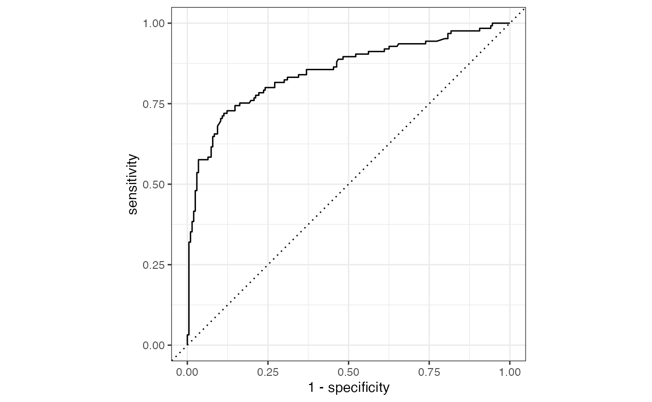
lr_test_pred |> conf_mat(truth = survived, estimate = .pred_class)#> Truth
#> Prediction yes no
#> yes 93 30
#> no 32 173The test AUC (0.851) should be similar to the CV estimate. If it were much worse, it would be a warning sign (leakage in the CV, or a test set that differs from the training data). The fitted workflow inside lr_final can be extracted with extract_workflow(lr_final) and used with predict() on new passengers.
WarningCommon pitfalls
- Judging a model by its training error. It always improves with complexity. Use CV or a validation set.
- Preprocessing before splitting (scaling, imputing, selecting features on the full data). Put every data-dependent step inside the recipe.
- Using the test set more than once. As soon as you pick a model because of its test score, the test score is no longer an honest estimate.
- Reporting accuracy alone with imbalanced classes. Compare with the majority-class baseline and look at sensitivity, specificity and AUC.
- Forgetting which level is the event. yardstick uses the first factor level by default; check
levels(df$outcome). - Over-interpreting small differences. Look at
std_err: two models whose CV AUCs differ by less than their standard errors are, practically, tied.
9. Check your understanding
10. Exercises
★ Exercise 1 — baselines. (a) Compute by hand, on titanic_train, the accuracy of the rule “everybody dies”. (b) For a regression problem predicting fare, what is the baseline prediction, and what is its R² on the training data?
TipSolution
mean(titanic_train$survived == "no") # about 0.62- The baseline predicts the training mean of
farefor everybody. By the definition of R², its R² on the training data is exactly 0 (on new data it can be slightly negative).
★★ Exercise 2 — predict, then check. In the k-NN simulation of section 3, what happens to the test RMSE at the best \(k\) if you increase the training size from 50 to 500? And what happens to the best \(k\)? Run the code to check.
TipSolution
set.seed(44)
train_big <- sim_data(500)
k_values <- c(1, 3, 5, 10, 20, 40, 80, 150)
sapply(k_values, \(k) rmse_vec_base(
  test_big$y, knn_reg(train_big$x, train_big$y, test_big$x, k)))
With more data the best test RMSE gets closer to the noise level 0.3 (more data reduce variance), and the best \(k\) becomes larger (with more points, we can average over more neighbours without leaving the local region, so we can afford a smoother fit).
★★ Exercise 3 — debug the leakage. A colleague writes:
titanic_scaled <- titanic |>
  mutate(age = (age - mean(age, na.rm = TRUE)) / sd(age, na.rm = TRUE))
split <- initial_split(titanic_scaled, strata = survived)
What is wrong, and how would you rewrite it in tidymodels?
TipSolution
The mean and SD of age are computed on all passengers, including the future test set: test information leaks into training. Split first and put the scaling in a recipe:
split <- initial_split(titanic, strata = survived)
rec <- recipe(survived ~ ., data = training(split)) |>
  step_impute_median(age) |>
  step_normalize(age)
The recipe learns mean and SD from the training data (or the training fold) and applies those same numbers to the test data.
★★ Exercise 4 — interpret metrics. A screening model for a disease with prevalence 5% has accuracy 0.95, sensitivity 0.02, specificity 0.999 and ROC AUC 0.80. Write three sentences for a clinician.
TipSolution
The 95% accuracy is no better than declaring everybody healthy, which also gives 95%. At the current threshold the model misses almost every sick patient (it detects only 2% of them), so it is useless for screening as it stands. However, an AUC of 0.80 shows that it does rank sick patients higher than healthy ones most of the time, so lowering the threshold could give a useful sensitivity, at the cost of more false alarms.
★★★ Exercise 5 — a richer recipe. Add to titanic_rec a feature family = sibsp + parch (hint: step_mutate()), and an interaction between sex and class (hint: step_interact(terms = ~ starts_with("sex_"):starts_with("pclass_")) after step_dummy()). Compare the CV ROC AUC with that of the original workflow. Is the difference larger than the standard errors?
TipSolution
rec2 <- recipe(survived ~ ., data = titanic_train) |>
  step_mutate(family = sibsp + parch) |>
  step_impute_median(all_numeric_predictors()) |>
  step_impute_mode(all_nominal_predictors()) |>
  step_log(fare, offset = 1) |>
  step_dummy(all_nominal_predictors()) |>
  step_interact(terms = ~ starts_with("sex_"):starts_with("pclass_")) |>
  step_normalize(all_numeric_predictors())

set.seed(2026)
res2 <- fit_resamples(lr_wf |> update_recipe(rec2),
                      resamples = titanic_folds, metrics = titanic_metrics)
bind_rows(original = collect_metrics(lr_res),
          richer = collect_metrics(res2), .id = "recipe") |>
  filter(.metric == "roc_auc")
The sex × class interaction usually raises the AUC a little (being a woman helped much more in 1st and 2nd class than in 3rd). Compare the gain with std_err: if it is smaller than about one standard error, the evidence for the richer model is weak.
Summary
| Idea / function | What it is for |
|---|---|
| Training / validation / test | Fit / choose / report — the test set is used once |
initial_split(df, prop, strata) |
Train–test split, stratified on the outcome |
vfold_cv(train, v, strata) |
k-fold cross-validation folds |
recipe() + step_*() |
Preprocessing learned on training data only (no leakage) |
logistic_reg() \|> set_engine("glm") |
Model specification (what + which software) |
workflow() |
Recipe + model in one object |
fit_resamples(), collect_metrics() |
Resampled performance estimates |
metric_set() |
Choose the metrics to compute |
null_model() |
Baseline: majority class / mean |
last_fit(wf, split) |
Final fit on training, single evaluation on test |
- Training error is optimistic; generalisation error is what matters.
- Flexibility trades bias against variance; the best model is in between.
- Everything learned from data (including preprocessing) belongs inside the resampling.
- Choose metrics by purpose: ranking (AUC), calibrated probabilities (Brier, log-loss), decisions at a threshold (sensitivity, specificity) — and always beat a baseline.