library(dplyr)
library(ggplot2)The logic of hypothesis testing
Null hypotheses, p-values, errors and power — built from a simulation
Understand what a hypothesis test does by building a permutation test by hand, then connect it to the standard tests; learn about type I and II errors, power, effect size, multiple testing and how to read p-values correctly.
NoteLearning objectives
By the end of this lesson you will be able to:
- state a null and an alternative hypothesis and choose a test statistic;
- run a permutation test by simulation and compute its p-value;
- explain type I and type II errors, the significance level and power;
- compute power and sample size with
power.t.test()and by simulation; - recognise the multiple-testing problem and adjust p-values with
p.adjust(); - interpret a p-value correctly and explain its link with confidence intervals.
1. Why test at all?
The built-in PlantGrowth data record the dried weight of plants grown under a control condition and two treatments, 10 plants per group. Let us compare the control with treatment 2.
plants <- PlantGrowth |>
  filter(group %in% c("ctrl", "trt2")) |>
  droplevels()

group_means <- tapply(plants$weight, plants$group, mean)
group_means
#> ctrl trt2
#> 5.032 5.526obs_diff <- unname(group_means["trt2"] - group_means["ctrl"])
obs_diff#> [1] 0.494Plants under treatment 2 are heavier on average, by 0.494 units. But we only have 10 plants per group, and plants vary a lot. Could a difference this large appear just by chance, even if the treatment did nothing? A hypothesis test answers exactly this question.
2. The logic in four steps
- Hypotheses. The null hypothesis \(H_0\) is the “boring” explanation: the treatment has no effect; any difference is due to chance. The alternative \(H_1\): the treatment changes the mean weight.
- Test statistic. A number that measures how far the data are from what \(H_0\) predicts. Here: the difference in means.
- Null distribution. The values the statistic would take if \(H_0\) were true, over many hypothetical repetitions of the study.
- p-value. The proportion of the null distribution that is at least as extreme as what we observed. A small p-value means: if \(H_0\) were true, data like ours would be rare.
The hardest step is the third. We now build the null distribution with a simulation.
3. A permutation test, by hand
If the treatment has no effect, the labels “ctrl” and “trt2” are just arbitrary names: each plant would have had the same weight whatever label it received. So we can shuffle the labels at random, recompute the difference in means, and repeat many times. Each shuffle is one “world where \(H_0\) is true”.
set.seed(123)
perm_diffs <- replicate(10000, {
  shuffled <- sample(plants$group)          # shuffle the labels
  m <- tapply(plants$weight, shuffled, mean)
  unname(m["trt2"] - m["ctrl"])
})ggplot(tibble(diff = perm_diffs), aes(diff)) +
geom_histogram(bins = 40, fill = "grey70", colour = "white") +
geom_vline(xintercept = c(-obs_diff, obs_diff),
colour = "#D55E00", linewidth = 1) +
labs(x = "Difference in means (trt2 - ctrl) after shuffling",
y = "Number of shuffles")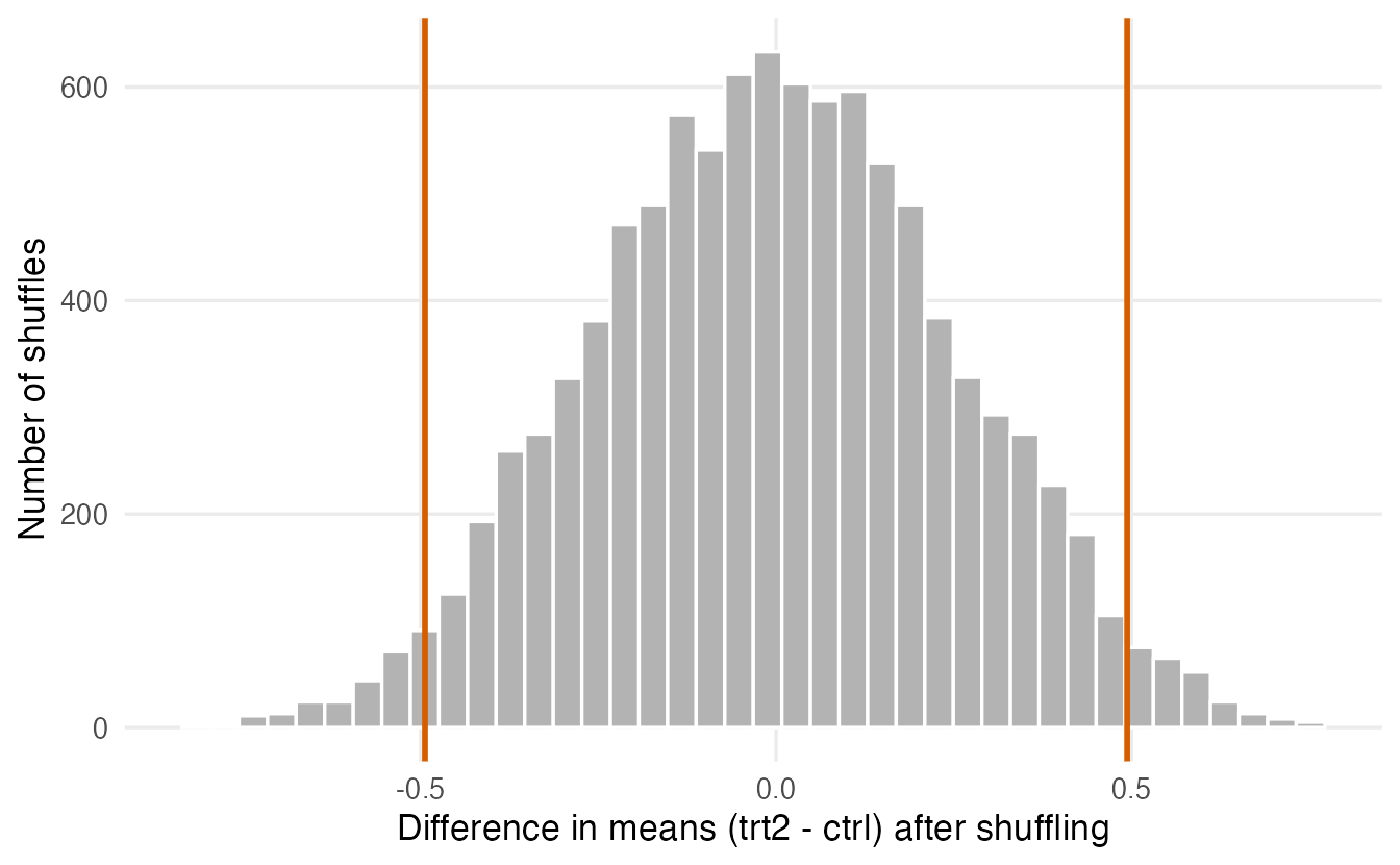
The histogram is centred on zero — as it should be under “no effect”. The observed difference sits out in the tail. How far out? We count:
p_perm <- mean(abs(perm_diffs) >= abs(obs_diff))
p_perm
#> [1] 0.0475
TipHow to read this result
Only 4.8% of the shuffled datasets gave a difference at least as large (in either direction) as the one we observed. This proportion is the p-value: 0.048. If the treatment did nothing, a difference of 0.49 or more (in either direction) would be unusual, but not extraordinary — roughly a 1-in-21 event.
4. The same answer from theory
Before computers, statisticians derived the null distribution mathematically. The two-sample t-test (see t-tests) assumes approximately normal data and uses the t distribution as the null distribution of the standardised difference.
t_res <- t.test(weight ~ group, data = plants, var.equal = TRUE)
t_res$p.value
#> [1] 0.04685The theoretical p-value (0.0469) is very close to the permutation p-value (0.0475). This is reassuring: the formula-based test is a shortcut for the simulation we just did. Permutation tests need fewer assumptions — essentially that, under \(H_0\), the labels are exchangeable — and we return to them in Non-parametric tests.
NoteGoing deeper: exact and Monte Carlo permutation tests
With 10 + 10 plants there are \(\binom{20}{10} =\) 184,756 ways to split the labels. Enumerating all of them gives the exact permutation p-value; sampling 10,000 of them gives a Monte Carlo approximation, with standard error about \(\sqrt{p(1-p)/10000}\) — here about 0.0021. A common refinement counts the observed split as one of the permutations: \((1 + \#\{\text{extreme}\}) / (1 + B)\), which guarantees the p-value is never exactly 0.
5. One-sided or two-sided?
So far \(H_1\) was “the means differ” (two-sided): we counted extreme values in both tails. If, before seeing the data, the only scientifically relevant question was “does treatment 2 increase weight?”, the alternative is one-sided and we count only the upper tail:
mean(perm_diffs >= obs_diff)#> [1] 0.0238t.test(weight ~ group, data = plants, var.equal = TRUE,
alternative = "less")$p.value#> [1] 0.02343The one-sided p-value is about half of the two-sided one. (In t.test() the difference is ctrl − trt2, following the order of the factor levels, so “trt2 is larger” means alternative = "less".)
WarningChoose the direction before looking at the data
Switching to a one-sided test after seeing which way the data point is a way of halving your p-value for free. That is not legitimate. Use two-sided tests unless the direction was fixed in advance and an effect in the other direction would genuinely be irrelevant.
6. Decisions, α, and two kinds of errors
Often we have to make a decision: act as if there is an effect, or not. We fix in advance a significance level \(\alpha\) (conventionally 0.05) and reject \(H_0\) if \(p \le \alpha\).
Any decision rule can go wrong in two ways:
| \(H_0\) true (no effect) | \(H_0\) false (real effect) | |
|---|---|---|
| Reject \(H_0\) | Type I error (false positive). Probability \(= \alpha\) | Correct: detection. Probability \(=\) power \(= 1 - \beta\) |
| Do not reject \(H_0\) | Correct | Type II error (false negative). Probability \(= \beta\) |
The courtroom analogy. A defendant is presumed innocent (\(H_0\)) until proven guilty beyond reasonable doubt.
- Convicting an innocent person is a type I error. The legal system keeps it rare by demanding strong evidence (a small \(\alpha\)).
- Acquitting a guilty person is a type II error. It happens when the evidence is too weak — for example, too few witnesses (a small sample).
- “Not guilty” does not mean “innocent”. Likewise, “not significant” does not mean “no effect”; it means the evidence was not strong enough.
Lowering \(\alpha\) protects against false positives but, for the same data, makes false negatives more likely. The only way to reduce both is to collect more (or better) data.
7. Power: will my study detect a real effect?
Power is the probability that the test rejects \(H_0\) when a real effect of a given size exists. It depends on:
- the effect size — how large the true difference is relative to the noise. A common measure is Cohen’s \(d\), the difference in means divided by the standard deviation (see t-tests);
- the sample size \(n\);
- the significance level \(\alpha\).
Power by simulation
Suppose the true effect is \(d = 0.5\) (a “medium” effect) and we plan 20 subjects per group. We simulate many studies and count how often the test is significant:
set.seed(1)
p_vals <- replicate(2000, {
  control <- rnorm(20, mean = 0,   sd = 1)
  treated <- rnorm(20, mean = 0.5, sd = 1)
  t.test(treated, control)$p.value
})
power_sim <- mean(p_vals < 0.05)
power_sim
#> [1] 0.3275Power with a formula
power.t.test(n = 20, delta = 0.5, sd = 1, sig.level = 0.05)#>
#> Two-sample t test power calculation
#>
#> n = 20
#> delta = 0.5
#> sd = 1
#> sig.level = 0.05
#> power = 0.3377
#> alternative = two.sided
#>
#> NOTE: n is number in *each* groupBoth approaches agree: with 20 per group, a medium effect is detected only about 33% of the time. Most studies would miss a real effect. Leave out n and set power instead to find the sample size you need:
ss <- power.t.test(power = 0.80, delta = 0.5, sd = 1)
ceiling(ss$n)
#> [1] 64To reach the conventional 80% power for \(d = 0.5\), you need about 64 subjects per group.
TipHow to read
power.t.test()
Give it all but one of n, delta, sd, sig.level, power, and it computes the missing one. delta is the true difference you want to detect, in the same units as sd; n is the size of each group (see the NOTE line). The hardest part is not the code but choosing a realistic delta: base it on previous studies or on the smallest difference that would matter in practice.
8. Statistical significance is not practical importance
With a large enough sample, even a negligible difference becomes “significant”. Imagine two very large groups whose true means differ by half a point on a scale with SD 15 (like an IQ test):
set.seed(3)
group_a <- rnorm(20000, mean = 100,   sd = 15)
group_b <- rnorm(20000, mean = 100.5, sd = 15)
t.test(group_a, group_b)$p.value
#> [1] 1.104e-07(mean(group_b) - mean(group_a)) / sd(c(group_a, group_b)) # rough Cohen's d#> [1] 0.05308The p-value is tiny, yet the effect size is about 0.05 standard deviations — practically irrelevant. The p-value tells you whether an effect is detectable, not whether it is large. Always report the estimated effect with its confidence interval.
9. Multiple testing: looking in many places
If you run one test at \(\alpha = 0.05\) on a true null, you have a 5% chance of a false positive. If you run 20 independent tests on true nulls, the chance of at least one false positive is \(1 - 0.95^{20} =\) 0.64.
Let us simulate 20 comparisons in which nothing is going on:
set.seed(28)
p20 <- replicate(20, t.test(rnorm(15), rnorm(15))$p.value)
round(sort(p20), 3)
#> [1] 0.005 0.006 0.039 0.064 0.076 0.152 0.160 0.160 0.369 0.624 0.652 0.655
#> [13] 0.723 0.798 0.823 0.849 0.933 0.972 0.981 0.985sum(p20 < 0.05)#> [1] 33 of the 20 “studies” look significant, although all the data are pure noise. Reporting only those would be misleading. (In fact, under \(H_0\) the p-value is uniformly distributed between 0 and 1, so about 1 in 20 falls below 0.05 by construction.)
The remedy is to adjust the p-values for the number of tests:
p_adj <- tibble(
  raw        = p20,
  bonferroni = p.adjust(p20, method = "bonferroni"),
  holm       = p.adjust(p20, method = "holm"),
  BH         = p.adjust(p20, method = "BH")
)
p_adj |> arrange(raw) |> head(5)
#> # A tibble: 5 × 4
#> raw bonferroni holm BH
#> <dbl> <dbl> <dbl> <dbl>
#> 1 0.004781 0.09563 0.09563 0.06442
#> 2 0.006442 0.1288 0.1224 0.06442
#> 3 0.03875 0.7751 0.6976 0.2584
#> 4 0.06424 1 1 0.3031
#> 5 0.07579 1 1 0.3031colSums(p_adj < 0.05)#> raw bonferroni holm BH
#> 3 0 0 0
TipHow to read this output
- Bonferroni multiplies each p-value by the number of tests (capped at 1). Simple, but conservative.
- Holm is a step-down version of Bonferroni: it controls the same error (the probability of any false positive, the family-wise error rate) and is never less powerful. There is no reason to prefer Bonferroni over Holm.
- BH (Benjamini–Hochberg) controls the false discovery rate: the expected proportion of false positives among the results you call significant. It is less strict and is popular when many tests are run (genomics, screening).
- Compare adjusted p-values with the usual \(\alpha\): after adjustment, the spurious “discoveries” disappear here.
10. What a p-value is — and is not
In 2016 the American Statistical Association published a statement on p-values (Wasserstein & Lazar, The American Statistician). Its six principles, in plain words:
- A p-value measures how incompatible the data are with a specified model (such as \(H_0\)).
- It is not the probability that \(H_0\) is true, nor the probability that the data were produced by chance alone.
- Scientific decisions should not rest only on whether \(p\) crosses a threshold such as 0.05.
- Proper inference requires full reporting and transparency: all tests run, not just the significant ones.
- A p-value does not measure the size or the importance of an effect.
- By itself, a p-value is not a good measure of evidence for a model or hypothesis.
Some common misreadings of “\(p = 0.03\)”:
| Statement | Correct? |
|---|---|
| “If \(H_0\) were true, data at least this extreme would occur about 3% of the time.” | ✅ Yes |
| “There is a 3% probability that \(H_0\) is true.” | ❌ No — the calculation assumes \(H_0\) is true |
| “There is a 97% probability that the effect is real.” | ❌ No |
| “The effect is large.” | ❌ Not implied — see Section 8 |
| “\(p = 0.06\) shows there is no effect.” | ❌ No — absence of evidence is not evidence of absence |
11. Tests and confidence intervals: two views of one calculation
A 95% confidence interval contains exactly those values that a two-sided test at \(\alpha = 0.05\) would not reject. Let us check with the plant data:
ci <- t_res$conf.int
ci
#> [1] -0.980338 -0.007662
#> attr(,"conf.level")
#> [1] 0.95# test H0: (ctrl - trt2) = d0 for several values d0
d0 <- c(-1.2, -1, -0.5, 0, 0.2)
p_d0 <- sapply(d0, \(d) {
t.test(weight ~ group, data = plants, var.equal = TRUE, mu = d)$p.value
})
tibble(d0, p = round(p_d0, 3), inside_ci = d0 >= ci[1] & d0 <= ci[2])#> # A tibble: 5 × 3
#> d0 p inside_ci
#> <dbl> <dbl> <lgl>
#> 1 -1.2 0.007 FALSE
#> 2 -1 0.042 FALSE
#> 3 -0.5 0.98 TRUE
#> 4 0 0.047 FALSE
#> 5 0.2 0.008 FALSEEvery value inside the interval has \(p > 0.05\); every value outside has \(p < 0.05\). Because \(0\) lies just outside the interval, the test of “no difference” gives \(p\) just below 0.05. This is why a CI is more informative than a p-value alone: it shows all the values compatible with the data at once.
WarningCommon pitfalls
- Reading the p-value as the probability that \(H_0\) is true. It is computed assuming \(H_0\).
- Treating “not significant” as “no effect”. Check the CI and the power: a small study can easily miss a real effect.
- Choosing one-sided after looking at the data, or trying several tests and reporting the one that “works” (p-hacking).
- Running many tests without adjustment and reporting only the significant ones.
- Equating significance with importance. Report the effect size and its CI.
- Treating 0.05 as a magic line. \(p = 0.049\) and \(p = 0.051\) carry practically the same evidence.
12. Check your understanding
13. Exercises
Interactive (run in your browser)
★★ Exercise 1 — your own permutation test. Do manual cars (am == 1) have a different mean mpg from automatic cars (am == 0)? Complete the permutation test and compare its p-value with t.test().
Shuffle the transmission labels mtcars$am, and compare the shuffled differences with the observed difference obs.
perm <- replicate(5000, {
  am_shuffled <- sample(mtcars$am)
  mean(mtcars$mpg[am_shuffled == 1]) - mean(mtcars$mpg[am_shuffled == 0])
})
mean(abs(perm) >= abs(obs))
The observed difference is about 7.2 mpg. Only a handful of the 5,000 shuffles reach it, so the permutation p-value is well below 0.01 (about 0.0006 with this seed), in line with the t-test (p ≈ 0.0003). If no shuffle at all reaches the observed value, do not report “p = 0” but “p < 1/5000”.
★ Exercise 2 — plan a study. You expect a difference of 5 units between two groups, with a standard deviation of 12. (a) What power do you have with 30 subjects per group? (b) How many per group do you need for 90% power?
delta is the expected difference (5) and sd the standard deviation (12). Power is a number between 0 and 1.
power.t.test(n = 30, delta = 5, sd = 12)        # power about 0.35
power.t.test(power = 0.90, delta = 5, sd = 12)  # n = 122.01, so 123 per group
With 30 per group the study would miss the effect about two times out of three. About 123 subjects per group (always round up) are needed for 90% power — a sobering but very common result.
★★ Exercise 3 — adjust for multiple testing. A screening study reports these eight p-values. How many are below 0.05 before adjustment, after Holm, and after BH?
The method names are "holm" and "BH".
sum(p < 0.05)                              # 6
sum(p.adjust(p, method = "holm") < 0.05)   # 1
sum(p.adjust(p, method = "BH") < 0.05)     # 3
Holm controls the chance of any false positive and keeps only the smallest p-value. BH controls the expected proportion of false discoveries and keeps three: it is less strict. Which one to use depends on the cost of a false positive.
Practice on your own computer
★★★ Exercise 4 — a power curve. Using simulation (1,000 replicates per point), estimate the power of a two-sample t-test for a true effect \(d = 0.5\) with \(n = 10, 20, 40, 80\) per group. Plot power against \(n\) and add the values from power.t.test().
TipSolution
set.seed(42)
sim_power <- function(n, d, reps = 1000) {
  mean(replicate(reps, t.test(rnorm(n, d), rnorm(n, 0))$p.value < 0.05))
}
pw <- tibble(n = c(10, 20, 40, 80)) |>
  mutate(
    simulated = sapply(n, sim_power, d = 0.5),
    formula   = sapply(n, \(k) power.t.test(n = k, delta = 0.5)$power)
  )
pw

ggplot(pw, aes(n, simulated)) +
  geom_line(linewidth = 1) +
  geom_point(aes(y = formula), colour = "#D55E00", size = 3) +
  geom_hline(yintercept = 0.8, linetype = "dashed") +
  labs(x = "n per group", y = "Power", title = "Power for d = 0.5")
Power grows from about 0.18 (n = 10) to about 0.88 (n = 80); the simulated and formula values agree within simulation error. The 80% line is crossed between 40 and 80 per group (≈ 64, as found in Section 7).
★★ Exercise 5 — interpret. A paper reports: “The new teaching method improved exam scores (p = 0.04, n = 2,000 per group). The mean difference was 0.6 points on a 100-point scale (95% CI 0.03 to 1.2).” Write three sentences for a school board: is the result real, is it important, and what is still uncertain?
TipSolution
A difference this large would be fairly unusual if the method had no effect (p = 0.04), so there is some evidence of a real effect. However, the estimated improvement is tiny — less than one point out of 100 — and even the upper end of the interval (1.2 points) is small, so the practical benefit is doubtful. The interval also reaches almost zero, so the true effect could be negligible; the decision should weigh costs and other outcomes, not the p-value alone.
Summary
| Idea / function | What it does |
|---|---|
| \(H_0\), \(H_1\) | The “no effect” model and its alternative |
Permutation test (sample() + replicate()) |
Builds the null distribution by shuffling labels |
| p-value | Probability, under \(H_0\), of data at least as extreme as observed |
| \(\alpha\) | Pre-chosen type I error rate (false-positive rate) |
Power, power.t.test() |
Probability of detecting a true effect; sample size planning |
p.adjust(p, "holm"), "BH" |
Adjusting for multiple tests |
- A test compares the observed statistic with its null distribution; a simulation makes that distribution visible.
- Small p-value: data are surprising if \(H_0\) were true — nothing more.
- Non-significant ≠ no effect; significant ≠ important. Report effect sizes and CIs.
- Plan studies with enough power; adjust when you run many tests.
- A 95% CI contains exactly the values not rejected at \(\alpha = 0.05\).