Autoencoders

Networks that learn to compress — for representation, denoising and spotting unusual cases

Build an autoencoder with keras3 on the wholesale-customers data: encoder, bottleneck and decoder, reconstruction error, comparison with PCA, a denoising variant and reconstruction-based anomaly detection.

Level 4 · Models & learning ⏱ ~75 min Prerequisites: DNNs for tabular data, PCA

Learning objectives

By the end of this lesson you will be able to:

describe an autoencoder as encoder + bottleneck + decoder trained to reproduce its own input;
explain why a linear autoencoder is closely related to PCA, and use PCA as a baseline;
build an autoencoder and a separate encoder with the keras3 functional API;
compute reconstruction errors and use them, with caution, to flag unusual observations;
train a denoising autoencoder.

library(dplyr)
library(readr)
library(ggplot2)

library(keras3)

Running this lesson

The model chunks need keras3 and a backend (see lesson 61). The results on this page were computed once and frozen. Without keras, the keras code is shown but not run, and numbers that depend on it read “not computed”. The PCA parts run in plain R.

1. Why learn to copy?

A wholesale distributor has 440 clients (hotels, restaurants, cafés and shops) and knows how much each spent in a year on six product categories. Two questions:

Can we summarise each client by two numbers that keep most of the information, to draw a map of clients?
Which clients have a spending profile that does not look like anyone else’s — possible data errors, or customers who deserve a closer look?

PCA (lesson 50) answers the first question with straight lines. An autoencoder answers both with a neural network that is trained to do something that sounds pointless: reproduce its own input.

2. The idea: squeeze, then rebuild

An autoencoder has two halves:

the encoder maps an input $x$ (6 numbers here) to a short code $z$ (2 numbers): $z = E(x)$;
the decoder tries to rebuild the input from the code: $\hat x = D(z)$.

The narrow middle layer is the bottleneck. Because it is narrow, the network cannot just copy $x$; it has to learn which combinations of the inputs matter. Training minimises the reconstruction error

\[ e(x) = \lVert x - D(E(x))\rVert^2 = \sum_{j=1}^{p}(x_j - \hat x_j)^2 , \]

averaged over the training rows. No outcome variable is needed: this is unsupervised learning, like PCA and clustering.

  x (6)  →  16  →  8  →  [ z (2) ]  →  8  →  16  →  x̂ (6)
  └──────── encoder ────────┘ bottleneck └──────── decoder ────────┘

Once trained, the encoder alone gives a 2-D representation, and the reconstruction error of a new row tells us how typical it is: rows that resemble the training data are rebuilt well; unusual rows are rebuilt badly.

Going deeper: a linear autoencoder is PCA

If encoder and decoder are linear ($z = Ax$, $\hat x = Bz$, with $A$ of size $d\times p$) and the loss is squared error, the best possible reconstruction projects $x$ onto the subspace spanned by the first $d$ principal components (Eckart–Young theorem). The network’s weights need not equal the PCA loadings — any basis of the same subspace is equally good — but the reconstructions and the error are the same. Non-linear activations let the autoencoder fit curved low-dimensional structure, which PCA cannot. That is also why PCA is the natural baseline: if the autoencoder does not reconstruct better than PCA with the same number of dimensions, the extra complexity has bought nothing.

3. Data and an honest split

wholesale <- read_csv(data_path("wholesale_customers.csv"),
                      show_col_types = FALSE)
spend_vars <- c("Fresh", "Milk", "Grocery", "Frozen",
                "Detergents_Paper", "Delicassen")
summary(wholesale[spend_vars])

#>      Fresh             Milk          Grocery          Frozen     
#>  Min.   :     3   Min.   :   55   Min.   :    3   Min.   :   25  
#>  1st Qu.:  3128   1st Qu.: 1533   1st Qu.: 2153   1st Qu.:  742  
#>  Median :  8504   Median : 3627   Median : 4756   Median : 1526  
#>  Mean   : 12000   Mean   : 5796   Mean   : 7951   Mean   : 3072  
#>  3rd Qu.: 16934   3rd Qu.: 7190   3rd Qu.:10656   3rd Qu.: 3554  
#>  Max.   :112151   Max.   :73498   Max.   :92780   Max.   :60869  
#>  Detergents_Paper   Delicassen   
#>  Min.   :    3    Min.   :    3  
#>  1st Qu.:  257    1st Qu.:  408  
#>  Median :  816    Median :  966  
#>  Mean   : 2881    Mean   : 1525  
#>  3rd Qu.: 3922    3rd Qu.: 1820  
#>  Max.   :40827    Max.   :47943

Spending is strongly right-skewed (a few huge clients), so we work on $\log(1 + x)$. Even without an outcome we need a validation set: an autoencoder can overfit, memorising the training clients instead of learning general structure. We split first and then standardise with the training means and standard deviations. (The original lesson standardised all rows before splitting; this small leak is fixed here.)

X_log <- log1p(as.matrix(wholesale[, spend_vars]))

set.seed(123)
idx_train <- sample(nrow(X_log), size = round(0.8 * nrow(X_log)))

mu <- colMeans(X_log[idx_train, ])
s  <- apply(X_log[idx_train, ], 2, sd)
standardise <- function(X) sweep(sweep(X, 2, mu, "-"), 2, s, "/")

x_train <- standardise(X_log[idx_train, ])
x_valid <- standardise(X_log[-idx_train, ])
x_all   <- standardise(X_log)            # all clients, training scale
c(train = nrow(x_train), valid = nrow(x_valid))

#> train valid 
#>   352    88

4. The linear baseline: PCA reconstruction

PCA with $k$ components is a linear encoder (the scores) plus a linear decoder (scores × loadings). We fit it on the training clients and measure the reconstruction error on the validation clients.

pca <- prcomp(x_train)
pca_reconstruct <- function(X, k) {
  scores <- predict(pca, X)[, 1:k, drop = FALSE]
  scores %*% t(pca$rotation[, 1:k, drop = FALSE])
}
recon_error <- function(X, X_hat) rowSums((X - X_hat)^2)

pca_err_by_k <- sapply(1:6, \(k) mean(recon_error(x_valid,
                                                  pca_reconstruct(x_valid, k))))
round(pca_err_by_k, 3)

#> [1] 2.751 1.298 0.901 0.349 0.106 0.000

How to read this output

Each number is the mean squared reconstruction error on the validation clients when keeping $k = 1, \dots, 6$ components. A client has 6 standardised values, so an error near 6 would mean “no better than predicting the average client”. With 2 components the error is 1.3; with all 6 it is zero (nothing is compressed). On the training clients the first two components explain 71% of the variance.

5. Building the autoencoder

We use the keras3 functional API: we describe how a tensor flows from an input through layers, then wrap the start and end points in keras_model(). Because the encoder is the first half of the same graph, we can define it as a second model that shares the layers.

build_autoencoder <- function(n_inputs, latent_dim = 2) {
  input <- keras_input(shape = n_inputs)
  latent <- input |>
    layer_dense(units = 16, activation = "relu") |>
    layer_dense(units = 8, activation = "relu") |>
    layer_dense(units = latent_dim, name = "latent")      # linear bottleneck
  output <- latent |>
    layer_dense(units = 8, activation = "relu") |>
    layer_dense(units = 16, activation = "relu") |>
    layer_dense(units = n_inputs)                         # linear output
  autoencoder <- keras_model(input, output)
  autoencoder |> compile(optimizer = optimizer_adam(learning_rate = 1e-3),
                         loss = "mse")
  list(autoencoder = autoencoder, encoder = keras_model(input, latent))
}

set_random_seed(123)
ae <- build_autoencoder(ncol(x_train))
ae$autoencoder

#> Model: "functional"
#> ┏━━━━━━━━━━━━━━━━━━━━━━━━━━━━━━━━━━━┳━━━━━━━━━━━━━━━━━━━━━━━━━━┳━━━━━━━━━━━━━━━┓
#> ┃ Layer (type)                      ┃ Output Shape             ┃       Param # ┃
#> ┡━━━━━━━━━━━━━━━━━━━━━━━━━━━━━━━━━━━╇━━━━━━━━━━━━━━━━━━━━━━━━━━╇━━━━━━━━━━━━━━━┩
#> │ input_layer (InputLayer)          │ (None, 6)                │             0 │
#> ├───────────────────────────────────┼──────────────────────────┼───────────────┤
#> │ dense (Dense)                     │ (None, 16)               │           112 │
#> ├───────────────────────────────────┼──────────────────────────┼───────────────┤
#> │ dense_1 (Dense)                   │ (None, 8)                │           136 │
#> ├───────────────────────────────────┼──────────────────────────┼───────────────┤
#> │ latent (Dense)                    │ (None, 2)                │            18 │
#> ├───────────────────────────────────┼──────────────────────────┼───────────────┤
#> │ dense_2 (Dense)                   │ (None, 8)                │            24 │
#> ├───────────────────────────────────┼──────────────────────────┼───────────────┤
#> │ dense_3 (Dense)                   │ (None, 16)               │           144 │
#> ├───────────────────────────────────┼──────────────────────────┼───────────────┤
#> │ dense_4 (Dense)                   │ (None, 6)                │           102 │
#> └───────────────────────────────────┴──────────────────────────┴───────────────┘
#>  Total params: 536 (2.09 KB)
#>  Trainable params: 536 (2.09 KB)
#>  Non-trainable params: 0 (0.00 B)

Design choices: ReLU in the hidden layers; a linear bottleneck and a linear output layer, because standardised data can be negative and a ReLU output could not produce negative values. The network is small (a few hundred weights) because we only have 352 training clients.

6. Training: the target is the input

The only unusual thing about fit() is that y is the same matrix as x.

early_stop <- callback_early_stopping(monitor = "val_loss", patience = 30,
                                      restore_best_weights = TRUE)
history <- ae$autoencoder |> fit(
  x = x_train, y = x_train,                       # reproduce the input
  validation_data = list(x_valid, x_valid),
  epochs = 500, batch_size = 32,
  callbacks = list(early_stop), verbose = 0
)

as.data.frame(history) |>
  filter(!is.na(value)) |>
  ggplot(aes(epoch, value, colour = data)) +
  geom_line(linewidth = 0.8) +
  labs(x = "Epoch", y = "MSE", colour = NULL)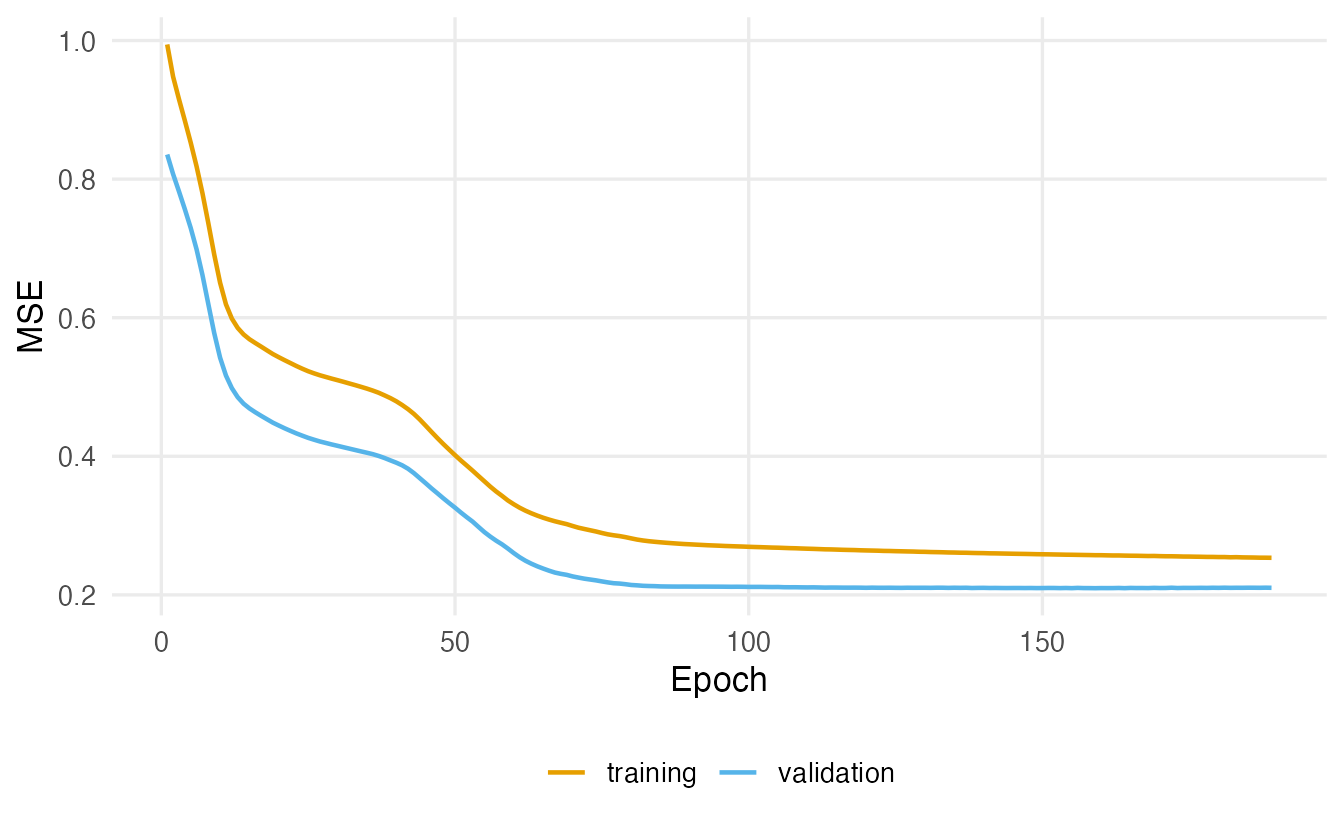

Figure 1: Training and validation reconstruction loss (mean squared error per value) of the autoencoder.

Now compare the validation reconstruction error with PCA using the same number of dimensions:

xhat_valid <- predict(ae$autoencoder, x_valid, verbose = 0)
c(pca_2 = mean(recon_error(x_valid, pca_reconstruct(x_valid, 2))),
  autoencoder_2 = mean(recon_error(x_valid, xhat_valid)))

#>         pca_2 autoencoder_2 
#>         1.298         1.258

How to read this output

Both numbers are mean squared errors per client on the validation set (6 values per client). Lower is better. The autoencoder’s error is 1.26, against 1.3 for 2-component PCA. With only 352 training rows and 6 variables, there is little curved structure to discover, so do not expect a big gain; if the autoencoder is worse, it has overfitted or not converged, and PCA is the better tool for these data.

7. The learned map of clients

The Channel variable (1 = hotel/restaurant/café, 2 = retail) was not used in training. If the 2-D code is meaningful, the two channels should occupy different regions.

z_all <- predict(ae$encoder, x_all, verbose = 0)
pc_all <- predict(pca, x_all)[, 1:2]
maps <- rbind(
  data.frame(d1 = z_all[, 1], d2 = z_all[, 2], method = "Autoencoder"),
  data.frame(d1 = pc_all[, 1], d2 = pc_all[, 2], method = "PCA")
)
maps$channel <- factor(rep(wholesale$Channel, 2), labels = c("Horeca", "Retail"))
ggplot(maps, aes(d1, d2, colour = channel)) +
  geom_point(alpha = 0.6) +
  facet_wrap(~ method, scales = "free") +
  labs(x = "dimension 1", y = "dimension 2", colour = "Channel")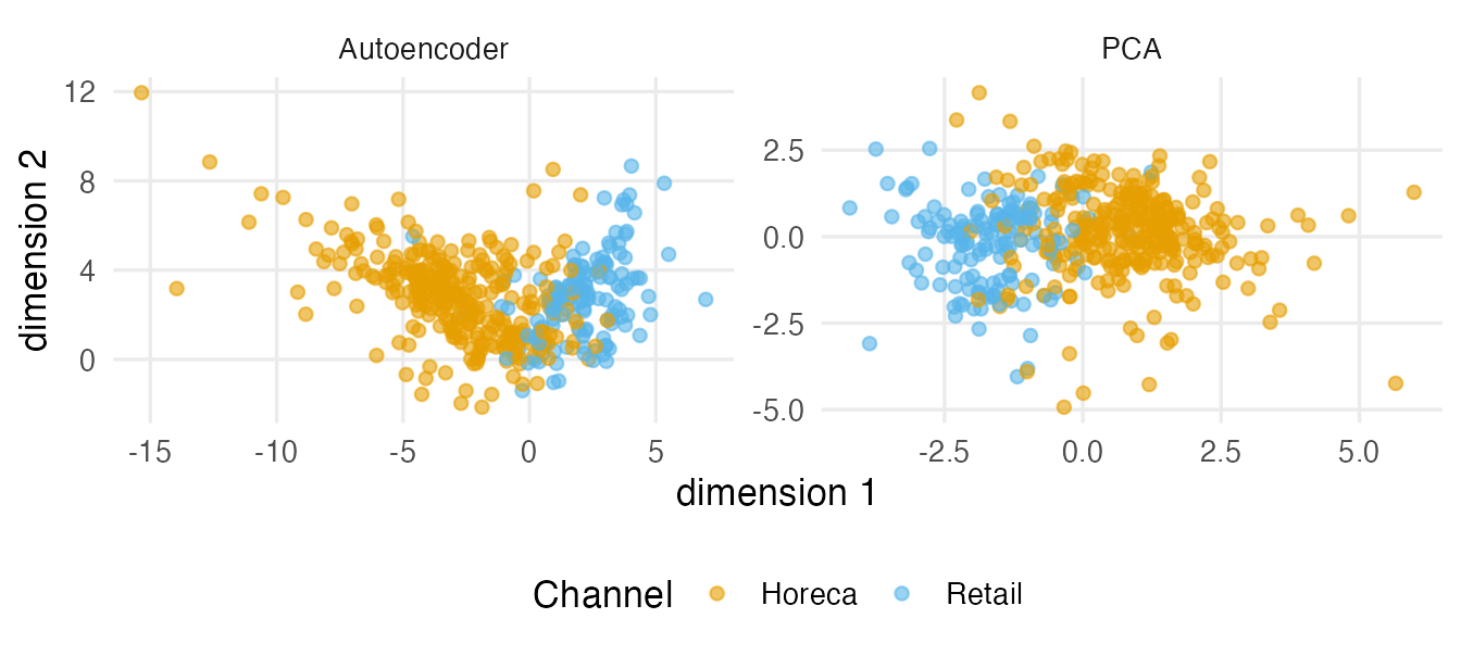

Figure 2: Clients in the 2-D code learned by the autoencoder (left) and in the first two principal components (right), coloured by sales channel, which neither method saw.

The autoencoder’s axes have no fixed meaning or orientation (another run may rotate or flip them), unlike PCA’s ordered components. To interpret them, correlate them with the original variables, e.g. cor(z_all, x_all).

8. Reconstruction error as an “unusualness” score

For each client, the reconstruction error measures how badly the model rebuilds it. We set a threshold at the 95th percentile of the training errors and flag clients above it.

err_ae  <- recon_error(x_all, predict(ae$autoencoder, x_all, verbose = 0))
err_pca <- recon_error(x_all, pca_reconstruct(x_all, 2))
thr_ae  <- quantile(err_ae[idx_train], 0.95)
thr_pca <- quantile(err_pca[idx_train], 0.95)
flag_ae  <- which(err_ae > thr_ae)
flag_pca <- which(err_pca > thr_pca)
c(flagged_ae = length(flag_ae), flagged_pca = length(flag_pca),
  both = length(intersect(flag_ae, flag_pca)))

#>  flagged_ae flagged_pca        both 
#>          20          19          15

wholesale |>
  mutate(error = round(err_ae, 1)) |>
  slice_max(error, n = 5) |>
  select(Channel, all_of(spend_vars), error)

#> # A tibble: 5 × 8
#>   Channel Fresh  Milk Grocery Frozen Detergents_Paper Delicassen error
#>     <dbl> <dbl> <dbl>   <dbl>  <dbl>            <dbl>      <dbl> <dbl>
#> 1       1     3   333    7021  15601               15        550  27.7
#> 2       1 37036  7152    8253   2995               20          3  19.2
#> 3       1     3  2920    6252    440              223        709  12.8
#> 4       1 20398  1137       3   4407                3        975  12  
#> 5       1  2438  8002    9819   6269             3459          3   8.3

How to read this output

The first table counts the clients flagged by each method and by both (15 in common). The second lists the five clients that the autoencoder reconstructs worst. Look at their raw spending: typically they combine a category with almost zero spending (values like 3 or 15) with normal spending elsewhere — a combination that is rare among the other clients. Whether that is a data-entry error or a genuinely special customer is a question for someone who knows the business, not for the model.

Reconstruction error is a score, not a verdict

An autoencoder trained on data that contain anomalies may learn to reconstruct them too.
The threshold (here the 95th percentile) is a choice, not a statistical test: it flags about 5% of clients by construction.
With few variables, simple alternatives (PCA reconstruction, robust z-scores, Mahalanobis distance) often flag almost the same rows. Use the autoencoder when the data are high-dimensional (e.g. images, sensor readings) and “normal” is a complex pattern.

9. A denoising autoencoder

A denoising autoencoder receives a corrupted input $\tilde x = x + \varepsilon$ but is asked to reproduce the clean $x$. It cannot succeed by copying; it must learn the structure that the noise destroys. This often gives more robust codes.

set.seed(1)
add_noise <- function(X, sd = 0.3) X + matrix(rnorm(length(X), sd = sd), nrow(X))
x_train_noisy <- add_noise(x_train)
x_valid_noisy <- add_noise(x_valid)

set_random_seed(123)
dae <- build_autoencoder(ncol(x_train))
history_dae <- dae$autoencoder |> fit(
  x = x_train_noisy, y = x_train,                 # noisy in, clean out
  validation_data = list(x_valid_noisy, x_valid),
  epochs = 500, batch_size = 32,
  callbacks = list(callback_early_stopping(monitor = "val_loss", patience = 30,
                                           restore_best_weights = TRUE)),
  verbose = 0
)
c(noisy_input = mean(recon_error(x_valid, x_valid_noisy)),
  denoised = mean(recon_error(x_valid, predict(dae$autoencoder, x_valid_noisy,
                                               verbose = 0))))

#> noisy_input    denoised 
#>      0.5303      1.2570

The first number is how far the noisy validation inputs are from the clean ones; the second is how far the denoised reconstructions are. (The noise uses R’s own random numbers, so set.seed() is the right tool for that line; the network uses set_random_seed().)

Common pitfalls

Skipping the validation set because “there is no outcome”. Autoencoders overfit too.
Standardising before splitting, or with statistics that include the validation rows.
A ReLU (or sigmoid) output layer for standardised data. It cannot produce negative values; use a linear output.
A bottleneck as wide as the input. Then the network can learn the identity and the code is useless.
Interpreting latent axes like principal components. They have no natural order, sign or scale.
Treating the top-5% reconstruction errors as “the anomalies”. It is a ranking; the cut-off and the follow-up are human decisions.

10. Check your understanding

Q1. Why must the bottleneck be smaller than the input?

Otherwise the network can reproduce the input by (approximately) copying it, minimising the loss without learning any structure. The narrow layer forces compression.

Q2. What is the target y in fit() for an ordinary autoencoder, and for a denoising one?

For both, the clean input x. The ordinary autoencoder receives x as input; the denoising one receives a corrupted version of x.

Q3. When would you expect an autoencoder to beat PCA clearly?

When the data are high-dimensional and lie near a curved (non-linear) low-dimensional structure, and there are enough observations to learn it — e.g. images. With 6 variables and a few hundred rows, PCA is usually as good.

11. Exercises

★ Exercise 1 — count the parameters. Without running code, compute the number of parameters of the autoencoder of Section 5 (6 → 16 → 8 → 2 → 8 → 16 → 6). Then check with ae$autoencoder.

Solution

$6\cdot16+16 = 112$; $16\cdot8+8 = 136$; $8\cdot2+2 = 18$; $2\cdot8+8 = 24$; $8\cdot16+16 = 144$; $16\cdot6+6 = 102$. Total $= 536$. The encoder alone has $112+136+18 = 266$.

★★ Exercise 2 — how many dimensions? Fit autoencoders with latent_dim = 1, 2, 3, 4 and plot the validation reconstruction error against the dimension, together with pca_err_by_k[1:4]. Where do the two curves differ most?

Solution

ae_err <- sapply(1:4, \(d) {
  set_random_seed(123)
  m <- build_autoencoder(ncol(x_train), latent_dim = d)
  m$autoencoder |> fit(x_train, x_train,
    validation_data = list(x_valid, x_valid), epochs = 500, batch_size = 32,
    verbose = 0, callbacks = list(callback_early_stopping(
      monitor = "val_loss", patience = 30, restore_best_weights = TRUE)))
  mean(recon_error(x_valid, predict(m$autoencoder, x_valid, verbose = 0)))
})
plot(1:4, pca_err_by_k[1:4], type = "b", ylim = c(0, max(pca_err_by_k)),
     xlab = "dimensions", ylab = "validation error")
lines(1:4, ae_err, type = "b", col = "steelblue")

Any gain of the autoencoder, if present, is usually largest for 1–2 dimensions, where a curved summary can capture more than a straight line. As the dimension grows both errors shrink towards 0 and the curves come together.

★★ Exercise 3 — plant an anomaly. Create a fake client with typical spending in every category except Grocery, which you set to the maximum observed value, and Detergents_Paper set to 3. Standardise it with standardise() (after log1p()) and compute its reconstruction error. Is it above thr_ae?

Solution

fake <- apply(X_log[idx_train, ], 2, median)
fake["Grocery"] <- max(X_log[, "Grocery"])
fake["Detergents_Paper"] <- log1p(3)
x_fake <- standardise(matrix(fake, nrow = 1, dimnames = list(NULL, spend_vars)))
recon_error(x_fake, predict(ae$autoencoder, x_fake, verbose = 0)) > thr_ae

In the data, grocery and detergents spending are strongly correlated; a client with very high grocery but almost no detergents breaks that pattern, so the error should be well above the threshold. This is the kind of anomaly an autoencoder (or PCA) can detect: a combination that is unusual, even when each single value is within the observed range.

★★ Exercise 4 — clusters in the code. Run kmeans() with 3 clusters (and nstart = 25) on z_all, and cross-tabulate the clusters with Channel. Repeat on the first two PCA scores. Which representation gives clusters more aligned with the sales channel?

Solution

set.seed(1)
km_ae  <- kmeans(z_all, centers = 3, nstart = 25)
km_pca <- kmeans(pc_all, centers = 3, nstart = 25)
table(ae = km_ae$cluster, channel = wholesale$Channel)
table(pca = km_pca$cluster, channel = wholesale$Channel)

Read the tables row by row: a cluster that is almost all channel 1 or all channel 2 is “aligned”. Both representations usually separate the channels to a similar degree, because the main structure (grocery/milk/detergents vs fresh/frozen) is roughly linear. See k-means for how to choose the number of clusters.

★★★ Exercise 5 — interpret, don’t compute. A colleague trains an autoencoder on all 440 clients, flags the top 5% reconstruction errors and writes in a report: “22 customers are fraudulent”. Give three reasons why this conclusion is not justified.

Solution

The 5% cut-off guarantees that about 22 clients are flagged whatever the data — it is a ranking, not evidence. (2) “Unusual” is not “fraudulent”: large hotels or specialist shops can have rare but legitimate profiles; no labelled fraud cases were used to validate the method. (3) The model was trained on the same clients it scores, so anomalies may have been partly learned (and there was no validation of the model). A defensible report would say “these clients have unusual spending combinations and should be reviewed”.

Summary

Idea / code	Meaning
Encoder $E$, decoder $D$, bottleneck	Compress to a short code, rebuild from it
Reconstruction error $\lVert x - \hat x\rVert^2$	Training loss; also an “unusualness” score
`keras_input()`, `keras_model(input, output)`	Functional API: build graphs, share layers between models
`fit(x, x, validation_data = list(xv, xv))`	Target equals input
`fit(x_noisy, x, ...)`	Denoising autoencoder
PCA with $k$ components	Linear autoencoder baseline

An autoencoder learns a compressed representation by trying to reproduce its input through a narrow bottleneck.
A linear autoencoder spans the same subspace as PCA; non-linear layers can capture curved structure.
Always split and standardise on the training set, and compare with PCA at the same dimension.
Reconstruction error ranks how typical each row is; flagged rows need human interpretation.