library(dplyr)
library(ggplot2)
library(broom)Poisson regression
Modelling counts: rate ratios, exposure offsets and overdispersion
Why ordinary regression fails for count data, how a Poisson GLM with a log link works, how to read coefficients as rate ratios, how to model rates with an offset, and what to do when the data are overdispersed (quasi-Poisson, negative binomial) or have too many zeros.
NoteLearning objectives
By the end of this lesson you will be able to:
- explain why
lm()is a poor choice for count outcomes (impossible predictions, variance that grows with the mean); - fit a Poisson regression with
glm(family = poisson)and interpret its coefficients as rate ratios with confidence intervals; - model rates (counts per unit of exposure) with an offset;
- detect overdispersion with the Pearson statistic and handle it with quasi-Poisson or negative binomial models;
- recognise when excess zeros call for a zero-inflated or hurdle model.
1. Why not just use lm() for counts?
Many outcomes are counts: the number of insects on a plant, of breaks in a length of yarn, of hospital admissions in a week, of goals in a match. Counts have three features that a straight line ignores:
- they are never negative;
- they are whole numbers (0, 1, 2, …);
- their spread grows with their mean: places with an average of 2 insects vary between 0 and 5, places with an average of 20 vary between 10 and 30.
Let us simulate counts whose average grows with a predictor \(x\) and fit an ordinary linear model:
set.seed(2026)
sim <- tibble::tibble(x = runif(100, 0, 10),
                      y = rpois(100, lambda = exp(-1 + 0.35 * x)))
m_lm <- lm(y ~ x, data = sim)
range(fitted(m_lm))
#> [1] -1.428 7.263sum(fitted(m_lm) < 0)#> [1] 16The linear model predicts negative counts for 16 of the 100 observations: an impossible answer.
ggplot(sim, aes(x, y)) +
  geom_jitter(height = 0.1, width = 0, alpha = 0.6) +
  geom_smooth(method = "lm", formula = y ~ x, se = FALSE,
              colour = "#D55E00") +
  geom_hline(yintercept = 0, linetype = 3) +
  labs(x = "x", y = "Count")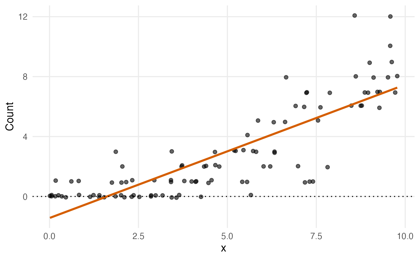
The second problem is visible in a real dataset. InsectSprays records the number of insects found on 72 agricultural plots treated with one of six insecticides (A to F), 12 plots each.
InsectSprays |>
  summarise(mean = mean(count), variance = var(count), .by = spray)
#> spray mean variance
#> 1 A 14.500 22.273
#> 2 B 15.333 18.242
#> 3 C 2.083 3.902
#> 4 D 4.917 6.265
#> 5 E 3.500 3.000
#> 6 F 16.667 38.606The sprays with a high mean count (A, B, F) also have a much larger variance than those with a low mean (C, D, E). lm() assumes the same variance everywhere, so its standard errors and p-values would be wrong. We need a model built for counts.
2. The Poisson distribution
The Poisson distribution describes the number of events that happen in a fixed amount of time or space when events occur independently at a constant average rate \(\mu\) (you met it in Probability distributions). Its key property is
\[ \text{mean} = \text{variance} = \mu . \]
tidyr::expand_grid(mu = c(1, 4, 10), y = 0:20) |>
  mutate(prob = dpois(y, mu), mu = paste("mean =", mu)) |>
  ggplot(aes(y, prob)) +
  geom_col(width = 0.8) +
  facet_wrap(~ mu) +
  labs(x = "Count", y = "Probability")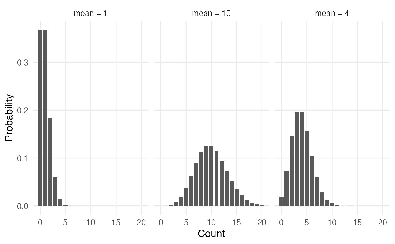
This “variance equals mean” property is exactly the pattern we saw in InsectSprays (roughly): Poisson regression builds it into the model instead of assuming a constant variance.
3. Poisson regression: a GLM with a log link
Like logistic regression, Poisson regression is a generalized linear model (GLM) with three ingredients:
- a distribution for \(y\): Poisson, with mean \(\mu\);
- a linear predictor: \(\eta = \beta_0 + \beta_1 x_1 + \dots + \beta_p x_p\);
- a link function connecting them: the logarithm, \(\log \mu = \eta\).
The log link guarantees that the predicted mean \(\mu = e^{\eta}\) is always positive, whatever the values of the predictors. It also makes effects multiplicative: adding 1 to \(x_1\) adds \(\beta_1\) to \(\log\mu\), so it multiplies \(\mu\) by \(e^{\beta_1}\).
Back to the simulated data:
m_sim <- glm(y ~ x, family = poisson, data = sim)
coef(m_sim)
#> (Intercept) x
#> -1.2050 0.3609exp(coef(m_sim))#> (Intercept) x
#> 0.2997 1.4347The estimates (-1.21 and 0.36) are close to the values used to simulate the data (\(-1\) and \(0.35\)). Each unit increase in \(x\) multiplies the expected count by about 1.43, i.e. an increase of about 43%. And all fitted values are positive:
sim |>
  mutate(fit_lm = fitted(m_lm), fit_pois = fitted(m_sim)) |>
  ggplot(aes(x, y)) +
  geom_jitter(height = 0.1, width = 0, alpha = 0.5) +
  geom_line(aes(y = fit_lm, colour = "lm"), linewidth = 1) +
  geom_line(aes(y = fit_pois, colour = "Poisson GLM"), linewidth = 1) +
  geom_hline(yintercept = 0, linetype = 3) +
  labs(x = "x", y = "Count", colour = NULL)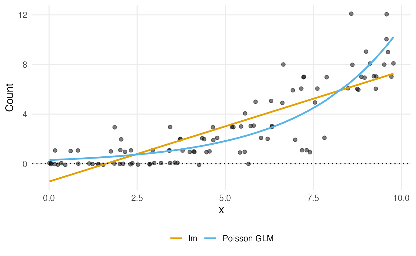
4. Fitting and reading a Poisson model
Do the insecticides differ in effectiveness?
ggplot(InsectSprays, aes(spray, count)) +
  geom_boxplot(outlier.shape = NA) +
  geom_jitter(width = 0.15, alpha = 0.5) +
  labs(x = "Spray", y = "Insects per plot")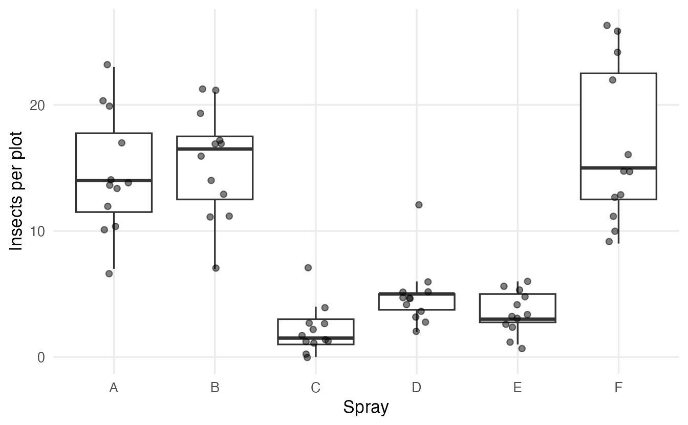
m_ins <- glm(count ~ spray, family = poisson, data = InsectSprays)
summary(m_ins)
#>
#> Call:
#> glm(formula = count ~ spray, family = poisson, data = InsectSprays)
#>
#> Coefficients:
#> Estimate Std. Error z value Pr(>|z|)
#> (Intercept) 2.6741 0.0758 35.27 <2e-16 ***
#> sprayB 0.0559 0.1057 0.53 0.60
#> sprayC -1.9402 0.2139 -9.07 <2e-16 ***
#> sprayD -1.0815 0.1507 -7.18 7e-13 ***
#> sprayE -1.4214 0.1719 -8.27 <2e-16 ***
#> sprayF 0.1393 0.1037 1.34 0.18
#> ---
#> Signif. codes: 0 '***' 0.001 '**' 0.01 '*' 0.05 '.' 0.1 ' ' 1
#>
#> (Dispersion parameter for poisson family taken to be 1)
#>
#> Null deviance: 409.041 on 71 degrees of freedom
#> Residual deviance: 98.329 on 66 degrees of freedom
#> AIC: 376.6
#>
#> Number of Fisher Scoring iterations: 5
TipHow to read this output
- Coefficients are on the log scale. Spray A is the reference level. The intercept, 2.67, is the log of the mean count for spray A: \(e^{2.674} = 14.5\), exactly the sample mean of group A.
sprayC= -1.94: the log of the mean count is 1.94 lower for spray C than for spray A. Negative = fewer insects.z value,Pr(>|z|): Wald tests of \(H_0: \beta = 0\) (no difference from spray A).- Dispersion parameter for poisson family taken to be 1: the model assumes variance = mean. We will check this in Section 7.
- Null / Residual deviance: lack of fit of the intercept-only model and of our model, as in logistic regression. The drop from 409 to 98.3 shows that spray matters a lot.
5. Interpretation: rate ratios
Log counts are hard to think in. Exponentiating a coefficient gives a rate ratio (RR, also called incidence rate ratio): the factor by which the expected count is multiplied.
exp(coef(m_ins))#> (Intercept) sprayB sprayC sprayD sprayE sprayF
#> 14.5000 1.0575 0.1437 0.3391 0.2414 1.1494exp(confint(m_ins)) # profile-likelihood 95% CIs, then exponentiated#> 2.5 % 97.5 %
#> (Intercept) 12.45083 16.7624
#> sprayB 0.85954 1.3015
#> sprayC 0.09225 0.2141
#> sprayD 0.25043 0.4525
#> sprayE 0.17019 0.3345
#> sprayF 0.93836 1.4093- Spray C vs A: RR = 0.14 (95% CI 0.09 to 0.21). Plots treated with C have, on average, 0.14 times as many insects as plots treated with A — about 86% fewer.
- Spray F vs A: RR = 1.15, with a CI that includes 1: no clear difference.
- RR = 1 means no difference; RR > 1 more events, RR < 1 fewer. A CI that excludes 1 corresponds to p < 0.05.
- The intercept’s exponentiated value is not a ratio: it is the expected count in the reference group.
With broom:
tidy(m_ins, exponentiate = TRUE, conf.int = TRUE)#> # A tibble: 6 × 7
#> term estimate std.error statistic p.value conf.low conf.high
#> <chr> <dbl> <dbl> <dbl> <dbl> <dbl> <dbl>
#> 1 (Intercept) 14.50 0.07581 35.27 1.448e-272 12.45 16.76
#> 2 sprayB 1.057 0.1057 0.5284 5.972e- 1 0.8595 1.302
#> 3 sprayC 0.1437 0.2139 -9.071 1.178e- 19 0.09225 0.2141
#> 4 sprayD 0.3391 0.1507 -7.179 7.029e- 13 0.2504 0.4525
#> 5 sprayE 0.2414 0.1719 -8.268 1.366e- 16 0.1702 0.3345
#> 6 sprayF 1.149 0.1037 1.343 1.792e- 1 0.9384 1.409Predicted counts come from predict(..., type = "response"); the default type = "link" returns the log of the expected count.
new_sprays <- tibble::tibble(spray = c("A", "C", "F"))
new_sprays |>
  mutate(expected = predict(m_ins, newdata = new_sprays, type = "response"))
#> # A tibble: 3 × 2
#> spray expected
#> <chr> <dbl>
#> 1 A 14.50
#> 2 C 2.083
#> 3 F 16.67
NoteGoing deeper: the Poisson likelihood
For counts \(y_i\) with means \(\mu_i = \exp(x_i^\top\beta)\), the probability of the data is \(\prod_i e^{-\mu_i}\mu_i^{y_i}/y_i!\), so the log-likelihood is
\[ \ell(\beta) = \sum_{i=1}^n \big[y_i \log\mu_i - \mu_i - \log(y_i!)\big]. \]
glm() maximises it by iteratively reweighted least squares. The deviance is
\[ D = 2\sum_{i=1}^n \Big[y_i \log\frac{y_i}{\hat\mu_i} - (y_i - \hat\mu_i)\Big], \]
twice the gap between the log-likelihood of a perfect (“saturated”) model and ours. As in logistic regression, the difference in deviance between nested models is approximately \(\chi^2\) with as many degrees of freedom as added parameters (likelihood-ratio test). With a categorical predictor only, the fitted means equal the group sample means.
6. Two factors and an interaction: warpbreaks
warpbreaks records the number of breaks in the warp yarn per loom, for two types of wool (A, B) and three levels of tension (L = low, M = medium, H = high), 9 looms per combination.
ggplot(warpbreaks, aes(tension, breaks, colour = wool)) +
  geom_jitter(width = 0.1, alpha = 0.6) +
  stat_summary(aes(group = wool), fun = mean, geom = "line",
               linewidth = 1) +
  labs(x = "Tension", y = "Breaks per loom", colour = "Wool")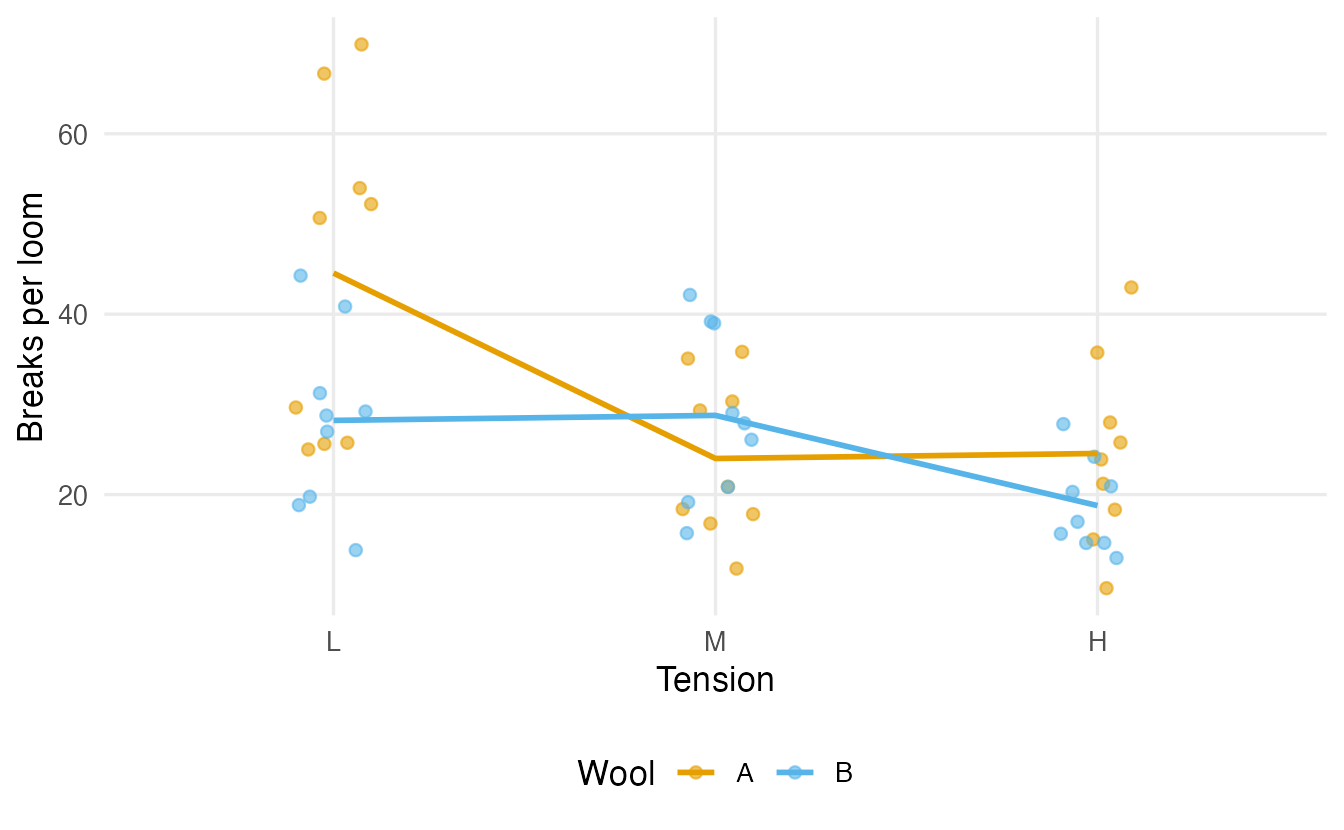
The lines are not parallel: going from low to medium tension reduces breaks a lot for wool A, but not for wool B. That suggests an interaction: the effect of tension depends on the wool. We compare the additive and the interaction model with a likelihood-ratio test:
m_add <- glm(breaks ~ wool + tension, family = poisson, data = warpbreaks)
m_int <- glm(breaks ~ wool * tension, family = poisson, data = warpbreaks)
anova(m_add, m_int, test = "Chisq")
#> Analysis of Deviance Table
#>
#> Model 1: breaks ~ wool + tension
#> Model 2: breaks ~ wool * tension
#> Resid. Df Resid. Dev Df Deviance Pr(>Chi)
#> 1 50 210
#> 2 48 182 2 28.1 8e-07 ***
#> ---
#> Signif. codes: 0 '***' 0.001 '**' 0.01 '*' 0.05 '.' 0.1 ' ' 1Taken at face value, the interaction is overwhelmingly significant. Keep this p-value in mind; we will revisit it in Section 7.
tidy(m_int, exponentiate = TRUE, conf.int = TRUE) |>
  select(term, rate_ratio = estimate, conf.low, conf.high) |>
  mutate(across(where(is.numeric), \(x) round(x, 2)))
#> # A tibble: 6 × 4
#> term rate_ratio conf.low conf.high
#> <chr> <dbl> <dbl> <dbl>
#> 1 (Intercept) 44.56 40.34 49.06
#> 2 woolB 0.63 0.54 0.74
#> 3 tensionM 0.54 0.46 0.63
#> 4 tensionH 0.55 0.47 0.65
#> 5 woolB:tensionM 1.89 1.49 2.41
#> 6 woolB:tensionH 1.21 0.94 1.56With an interaction, the main-effect rate ratios refer to the reference level of the other factor:
woolB= 0.63: at low tension, wool B has 0.63 times as many breaks as wool A.woolB:tensionM= 1.89: the wool B / wool A ratio at medium tension is 1.89 times the ratio at low tension, i.e. \(0.63 \times 1.89 = 1.2\). At medium tension wool B is slightly worse than A.
Interaction terms on a multiplicative scale are easy to misread. The clearest summary is a table of predicted counts:
wb_grid <- tidyr::expand_grid(wool = c("A", "B"), tension = c("L", "M", "H"))
wb_grid |>
  mutate(expected = predict(m_int, newdata = wb_grid, type = "response")) |>
  tidyr::pivot_wider(names_from = tension, values_from = expected)
#> # A tibble: 2 × 4
#> wool L M H
#> <chr> <dbl> <dbl> <dbl>
#> 1 A 44.56 24.00 24.56
#> 2 B 28.22 28.78 18.78Because the model has a parameter for each of the 6 combinations, these predictions equal the six sample means.
7. Overdispersion: when variance exceeds the mean
The Poisson model assumes that the variance equals the mean. Real counts are often more variable than that — for example because looms differ in ways we did not measure. This is overdispersion. If we ignore it, the model is overconfident: standard errors are too small, confidence intervals too narrow and p-values too small.
Checking with the Pearson statistic
A Pearson residual is \((y_i - \hat\mu_i)/\sqrt{\hat\mu_i}\): the raw residual divided by the standard deviation the Poisson model expects. If the model is right, the squared Pearson residuals average about 1, so
\[ \hat\phi = \frac{\sum_i r_i^2}{n - p} \approx 1, \]
where \(n - p\) is the residual degrees of freedom. Values clearly above 1 indicate overdispersion.
dispersion <- function(model) {
  sum(residuals(model, type = "pearson")^2) / df.residual(model)
}
dispersion(m_int)
#> [1] 3.764dispersion(m_ins)#> [1] 1.508For warpbreaks the estimated dispersion is 3.76: the variance is almost four times what the Poisson model assumes. For InsectSprays it is 1.51: milder, but still above 1.
How far from 1 is “clearly above”? A small simulation with data that really are Poisson shows the typical range:
set.seed(3)
disp_null <- replicate(500, {
  d <- data.frame(g = gl(3, 20))
  d$y <- rpois(60, lambda = c(3, 6, 9)[d$g])
  dispersion(glm(y ~ g, family = poisson, data = d))
})
quantile(disp_null, c(0.025, 0.5, 0.975))
#> 2.5% 50% 97.5%
#> 0.6748 0.9980 1.3947With 60 observations, genuine Poisson data give values between about 0.7 and 1.4. A value near 3.8 is far outside that range. (Formally, \(\sum r_i^2\) can be compared to a \(\chi^2_{n-p}\) distribution, but the ratio itself is the useful number: it tells you how much the standard errors are off.)
NoteOverdispersion or a missing predictor?
Before reaching for a new distribution, ask whether an important predictor is missing, or whether an interaction or a non-linear term is needed. Unexplained structure in the mean shows up as extra variance. Overdispersion models are for the variability that remains after the mean is modelled well.
Quasi-Poisson: inflate the standard errors
The simplest fix keeps the Poisson mean model but assumes \(\text{Var}(y) = \phi\,\mu\) and estimates \(\phi\) from the data:
m_qp <- glm(breaks ~ wool * tension, family = quasipoisson, data = warpbreaks)
summary(m_qp)$dispersion
#> [1] 3.764tibble::tibble(term = names(coef(m_int)),
estimate = coef(m_int),
se_poisson = sqrt(diag(vcov(m_int))),
se_quasi = sqrt(diag(vcov(m_qp))))#> # A tibble: 6 × 4
#> term estimate se_poisson se_quasi
#> <chr> <dbl> <dbl> <dbl>
#> 1 (Intercept) 3.797 0.04994 0.09688
#> 2 woolB -0.4566 0.08019 0.1556
#> 3 tensionM -0.6187 0.08440 0.1637
#> 4 tensionH -0.5958 0.08378 0.1625
#> 5 woolB:tensionM 0.6382 0.1222 0.2370
#> 6 woolB:tensionH 0.1884 0.1299 0.2520
TipHow to read this output
- The coefficients are identical: quasi-Poisson changes only the uncertainty, not the estimates.
- Every standard error is multiplied by \(\sqrt{\hat\phi} = 1.94\).
summary(m_qp)reports t tests instead of z tests, because \(\phi\) is estimated.
Models are now compared with an F-test (as in lm()), because the dispersion is estimated:
m_qp_add <- glm(breaks ~ wool + tension, family = quasipoisson,
                data = warpbreaks)
anova(m_qp_add, m_qp, test = "F")
#> Analysis of Deviance Table
#>
#> Model 1: breaks ~ wool + tension
#> Model 2: breaks ~ wool * tension
#> Resid. Df Resid. Dev Df Deviance F Pr(>F)
#> 1 50 210
#> 2 48 182 2 28.1 3.73 0.031 *
#> ---
#> Signif. codes: 0 '***' 0.001 '**' 0.01 '*' 0.05 '.' 0.1 ' ' 1The interaction is still supported, but the p-value is now 0.031 instead of 8e-07. The naive Poisson analysis overstated the evidence by several orders of magnitude.
Quasi-Poisson has no likelihood, so there is no AIC (AIC(m_qp) returns NA).
Negative binomial regression
The negative binomial distribution is a count distribution with an extra parameter \(\theta\) that lets the variance grow faster than the mean:
\[ \text{Var}(y) = \mu + \frac{\mu^2}{\theta}. \]
Small \(\theta\) means strong overdispersion; as \(\theta \to \infty\) it becomes the Poisson. It has a proper likelihood, so AIC and likelihood-ratio tests are available. It is fitted with glm.nb() from the MASS package (installed with R):
m_nb <- MASS::glm.nb(breaks ~ wool * tension, data = warpbreaks)
m_nb$theta
#> [1] 12.08AIC(m_int, m_nb)#> df AIC
#> m_int 6 469.0
#> m_nb 7 405.1tidy(m_nb, exponentiate = TRUE, conf.int = TRUE) |>
select(term, rate_ratio = estimate, conf.low, conf.high) |>
mutate(across(where(is.numeric), \(x) round(x, 2)))#> # A tibble: 6 × 4
#> term rate_ratio conf.low conf.high
#> <chr> <dbl> <dbl> <dbl>
#> 1 (Intercept) 44.56 36.19 55.32
#> 2 woolB 0.63 0.46 0.86
#> 3 tensionM 0.54 0.39 0.74
#> 4 tensionH 0.55 0.4 0.75
#> 5 woolB:tensionM 1.89 1.21 2.96
#> 6 woolB:tensionH 1.21 0.77 1.9The estimated \(\theta\) is 12.1 and AIC drops from 469 (Poisson) to 405.1: the negative binomial describes these data much better. Here the rate ratios are the same as in the Poisson fit (with a full set of group means, both models reproduce the six sample means), but the confidence intervals are wider.
NoteGoing deeper: quasi-Poisson or negative binomial?
Both allow extra variance, but in different shapes:
| Variance | Weights given to large counts | Likelihood / AIC | |
|---|---|---|---|
| Quasi-Poisson | \(\phi\,\mu\) (proportional to the mean) | as in Poisson | no |
| Negative binomial | \(\mu + \mu^2/\theta\) (grows quadratically) | smaller (large counts are noisier) | yes |
When the model contains continuous predictors, the two can give different coefficients, because they weight observations differently. A practical check is to group observations by fitted value and plot the observed variance against the mean: a straight line suggests quasi-Poisson, a curve bending upwards suggests the negative binomial. The negative binomial can be derived as a Poisson whose mean varies between units according to a gamma distribution — a model for unobserved heterogeneity.
The likelihood-ratio test of Poisson against negative binomial is non-standard (\(\theta = \infty\) is on the boundary of the parameter space), so comparing AIC, or simply looking at \(\hat\phi\), is the usual practice.
Why it matters: a coverage simulation
How bad is it to ignore overdispersion? We simulate 1000 studies with two groups of 30, true rate ratio 1.5, and negative-binomial (overdispersed) counts, and record how often the usual 95% Wald confidence interval for the rate ratio contains the true value:
set.seed(5)
cover <- replicate(1000, {
  g <- gl(2, 30, labels = c("a", "b"))
  y <- rnbinom(60, mu = ifelse(g == "a", 4, 6), size = 2)
  sapply(c("poisson", "quasipoisson"), \(fam) {
    m <- glm(y ~ g, family = fam)
    est <- coef(m)["gb"]
    se <- sqrt(vcov(m)["gb", "gb"])
    est - 1.96 * se < log(1.5) & log(1.5) < est + 1.96 * se
  })
})
rowMeans(cover)
#> poisson.gb quasipoisson.gb
#> 0.713 0.945The “95%” Poisson intervals contain the truth only 71% of the time; the quasi-Poisson intervals 94%. Ignoring overdispersion produces intervals that are too narrow and too many false discoveries.
8. Exposure and offsets: modelling rates
Often the units we count over have different sizes: clinics serve different numbers of patients, roads have different lengths, observation periods have different durations. A clinic with 8000 person-years of follow-up will see more cases than one with 500 simply because it is bigger. What we want to compare is the rate: cases per person-year.
We simulate 40 clinics. Urban clinics are large, rural clinics small, and the true rate is 2 cases per 1000 person-years in urban areas and 3 in rural areas (rate ratio 1.5).
set.seed(1)
n_cl <- 40
clinics <- tibble::tibble(
  area = factor(rep(c("urban", "rural"), each = n_cl / 2),
                levels = c("urban", "rural")),
  person_years = c(round(runif(n_cl / 2, 2000, 8000)),
                   round(runif(n_cl / 2, 200, 2000)))
)
true_rate <- ifelse(clinics$area == "urban", 2, 3) / 1000
clinics$cases <- rpois(n_cl, true_rate * clinics$person_years)

clinics |>
  summarise(cases = sum(cases), person_years = sum(person_years), .by = area)
#> # A tibble: 2 × 3
#> area cases person_years
#> <fct> <int> <dbl>
#> 1 urban 204 106620
#> 2 rural 63 21058A model of the raw counts answers the wrong question:
m_naive <- glm(cases ~ area, family = poisson, data = clinics)
exp(coef(m_naive))
#> (Intercept) arearural
#> 10.2000 0.3088It says that rural clinics have 0.31 times as many cases — because they are smaller, not because the risk is lower. To model the rate we write
\[ \log\frac{\mu_i}{t_i} = \beta_0 + \beta_1 x_i \quad\Longleftrightarrow\quad \log\mu_i = \log t_i + \beta_0 + \beta_1 x_i , \]
where \(t_i\) is the exposure (person-years). The term \(\log t_i\) enters the model with a coefficient fixed at 1: it is an offset, not a parameter to estimate.
m_rate <- glm(cases ~ area + offset(log(person_years)),
              family = poisson, data = clinics)
exp(coef(m_rate))
#> (Intercept) arearural
#> 0.001913 1.563623exp(confint(m_rate))#> 2.5 % 97.5 %
#> (Intercept) 0.001663 0.002188
#> arearural 1.169930 2.060551
TipHow to read this output
- Intercept: \(e^{\beta_0}\) = 0.0019 cases per person-year in urban clinics, i.e. 1.91 per 1000 person-years (true value: 2).
arearural: the rate ratio. Rural clinics have 1.56 times the rate of urban ones (95% CI 1.17 to 2.06; true value 1.5). The naive model had the direction wrong.- The offset does not appear in the coefficient table, because it has no coefficient.
Predictions need the exposure too. To get rates per 1000 person-years, predict for person_years = 1000:
new_cl <- tibble::tibble(area = c("urban", "rural"), person_years = 1000)
new_cl |>
  mutate(cases_per_1000 = predict(m_rate, newdata = new_cl,
                                  type = "response"))
#> # A tibble: 2 × 3
#> area person_years cases_per_1000
#> <chr> <dbl> <dbl>
#> 1 urban 1000 1.913
#> 2 rural 1000 2.992Two practical points:
- The offset must be on the log scale (because the link is log):
offset(log(person_years)), notoffset(person_years). - Entering
log(person_years)as an ordinary predictor (+ log(person_years)) is different: R would estimate its coefficient. That can be a useful check (an estimate close to 1 supports the “rate” assumption), but it is no longer a rate model.
9. Too many zeros
Sometimes the data contain many more zeros than a Poisson (or even a negative binomial) model predicts. Example: the number of cigarettes smoked yesterday — non-smokers always give 0, smokers give a count that is rarely 0. A first check is to compare the observed number of zeros with the number the fitted model expects, \(\sum_i P(Y_i = 0) = \sum_i e^{-\hat\mu_i}\):
c(observed = sum(InsectSprays$count == 0),
  expected = sum(dpois(0, fitted(m_ins))))
#> observed expected
#> 2.000 1.944For InsectSprays they agree well, so there is no excess of zeros. When there is, two families of models are common:
- Zero-inflated models: a mixture of a “structural zero” group (e.g. non-smokers) and a count model (which can also produce zeros);
- Hurdle models: one part models zero vs positive, a second part models the positive counts.
Both are available in the pscl package, with the same formula interface:
# count part | zero part
m_zip <- pscl::zeroinfl(y ~ x1 + x2 | x1, data = my_data, dist = "poisson")
m_hnb <- pscl::hurdle(y ~ x1 + x2 | x1, data = my_data, dist = "negbin")
The glmmTMB package also fits these models and adds random effects. Use them when the zeros have a plausible separate mechanism, not just because the data contain zeros: a Poisson with a small mean produces many zeros on its own.
WarningCommon pitfalls
- Using
lm()on counts (or onlog(y + 1)). Predictions can be negative, the variance is wrong, and back-transforming a log-mean is not the mean. - Reading coefficients as additive changes. They are on the log scale: exponentiate for rate ratios, and use predicted counts for absolute differences.
- Ignoring overdispersion. Always compute the Pearson dispersion. Values well above 1 make Poisson p-values far too small; use quasi-Poisson or negative binomial.
- Forgetting the exposure when units differ in size or observation time, or writing
offset(t)instead ofoffset(log(t)). - Comparing quasi-Poisson models with AIC or χ² tests. There is no likelihood: use
anova(..., test = "F"). - Misreading main effects in an interaction model. With
wool * tension, thewoolBrate ratio refers to the reference tension only. Report predicted counts for all combinations.
10. Check your understanding
11. Exercises
★ Exercise 1 — rate ratios. Refit m_ins with spray C as the reference level (hint: relevel()). Report the rate ratio of spray A versus C with its 95% CI, and write one sentence interpreting it.
TipSolution
ins_c <- InsectSprays |> mutate(spray = relevel(spray, ref = "C"))
m_c <- glm(count ~ spray, family = poisson, data = ins_c)
tidy(m_c, exponentiate = TRUE, conf.int = TRUE)
The RR for spray A vs C is about 7.0 (95% CI roughly 4.7 to 10.8): plots treated with A have about seven times as many insects as plots treated with C. It is simply \(1/0.144\) — changing the reference level inverts the ratio; the model is the same.
★★ Exercise 2 — interpret an output. From the coefficients of m_int, compute the rate ratio of wool B versus wool A at medium tension. Check your answer against the ratio of the two sample means.
TipSolution
b <- coef(m_int)
exp(b["woolB"] + b["woolB:tensionM"])

means <- with(warpbreaks, tapply(breaks, list(wool, tension), mean))
means["B", "M"] / means["A", "M"]
Both give about 1.20: at medium tension wool B has about 20% more breaks than wool A, while at low tension it has about 37% fewer (RR 0.63). The interaction is precisely this change in the ratio.
★★ Exercise 3 — overdispersion in InsectSprays. The dispersion of m_ins is about 1.5. Refit the model with family = quasipoisson. What happens to the coefficient and the standard error of sprayC? Does the conclusion “spray C is much more effective than A” change?
TipSolution
m_ins_qp <- glm(count ~ spray, family = quasipoisson, data = InsectSprays)
summary(m_ins_qp)$coefficients["sprayC", ]
exp(confint.default(m_ins_qp))["sprayC", ]
The coefficient is unchanged (\(-1.94\), RR 0.14); the standard error is multiplied by \(\sqrt{1.51} \approx 1.23\). The Wald 95% CI for the rate ratio widens to roughly 0.09–0.24, still far from 1. The conclusion stands; only the precision is more honest. (confint.default() gives Wald intervals, which work for quasi models.)
★★ Exercise 4 — debug. A colleague models the clinic data with
glm(cases ~ area + offset(person_years), family = poisson, data = clinics)and gets an error: no valid set of coefficients has been found. What is wrong? What would glm(cases ~ area + log(person_years), ...) estimate instead?
TipSolution
The offset must be on the scale of the linear predictor, which is the log of the mean: offset(log(person_years)). With offset(person_years) the model claims that \(\log\mu\) grows by 1 for every extra person-year, i.e. expected counts of order \(e^{8000}\), and the fitting algorithm cannot even start.
+ log(person_years) estimates a coefficient for log-exposure instead of fixing it at 1. For these simulated data the counts really are proportional to exposure, so the estimate should be compatible with 1 (it comes out at about 0.85, with a confidence interval that includes 1 — 40 clinics do not pin it down precisely). In real data, an estimate clearly different from 1 means that counts are not simply proportional to exposure.
★★ Exercise 5 — predict the output. In m_rate, suppose you measure exposure in thousands of person-years (py_k = person_years / 1000) and use offset(log(py_k)). Which coefficients change, and how? Check.
TipSolution
Only the intercept changes: \(\log(\mu) = \log(t/1000) + \beta_0' + \dots\) means \(\beta_0' = \beta_0 + \log(1000)\), so \(e^{\beta_0'}\) is the rate per 1000 person-years (about 1.9). The rate ratio for arearural is identical.
clinics <- clinics |> mutate(py_k = person_years / 1000)
m_rate_k <- glm(cases ~ area + offset(log(py_k)), family = poisson,
                data = clinics)
exp(coef(m_rate_k))
★★★ Exercise 6 — mini-analysis. Using warpbreaks, fit the additive model breaks ~ wool + tension with Poisson, quasi-Poisson and negative binomial. For each, report the rate ratio for high vs low tension with its 95% CI (use confint.default() for all three for a fair comparison). Which intervals would you trust, and why?
TipSolution
f <- breaks ~ wool + tension
fits <- list(
  poisson = glm(f, family = poisson, data = warpbreaks),
  quasi   = glm(f, family = quasipoisson, data = warpbreaks),
  negbin  = MASS::glm.nb(f, data = warpbreaks)
)
sapply(fits, \(m) exp(c(coef(m)["tensionH"],
                        confint.default(m)["tensionH", ])))
sapply(fits[c(1, 3)], AIC)
All three give a rate ratio of about 0.6 (roughly 40% fewer breaks at high tension). The Poisson interval is the narrowest; the quasi-Poisson and negative binomial intervals are about twice as wide. Since the Pearson dispersion of this model is well above 1 (about 4.3) the Poisson interval is too optimistic; the quasi-Poisson and negative binomial intervals are the ones to report, and AIC clearly prefers the negative binomial over the Poisson.
Summary
| Idea / function | What it does |
|---|---|
glm(y ~ x, family = poisson) |
Poisson regression, log link |
exp(coef(m)), exp(confint(m)) |
rate ratios and their CIs |
tidy(m, exponentiate = TRUE, conf.int = TRUE) |
rate-ratio table |
predict(m, newdata, type = "response") |
expected counts |
anova(m0, m1, test = "Chisq") |
likelihood-ratio test (Poisson, NB) |
offset(log(exposure)) |
model rates per unit of exposure |
sum(residuals(m, "pearson")^2) / df.residual(m) |
Pearson dispersion (≈ 1 for Poisson) |
glm(..., family = quasipoisson), anova(..., test = "F") |
inflate SEs for overdispersion |
MASS::glm.nb() |
negative binomial regression |
pscl::zeroinfl(), pscl::hurdle() |
models for excess zeros |
- Counts are non-negative and their variance grows with the mean: use a Poisson GLM with log link, not
lm(). - Exponentiated coefficients are rate ratios: multiplicative effects on the expected count.
- When units differ in size or observation time, model the rate with an offset.
- Always check overdispersion; if present, use quasi-Poisson or negative binomial — otherwise the p-values are far too small.
- Excess zeros with a separate mechanism call for zero-inflated or hurdle models.