Model-based clustering: Gaussian mixtures

Clusters as probability distributions — with soft memberships, elliptical shapes and BIC

Understand finite mixture models through a one-dimensional example, see the EM algorithm at work in a few lines of base R, fit Gaussian mixtures with mclust, read covariance models and BIC, use soft assignments and uncertainty, and compare with k-means.

Level 4 · Models & learning ⏱ ~90 min Prerequisites: Distributions, Clustering: the big picture, k-means

NoteLearning objectives

By the end of this lesson you will be able to:

• explain a finite mixture model and read the fitted component densities of a one-dimensional example;
• describe the EM algorithm (E-step and M-step) and run a small version of it in base R;
• fit Gaussian mixtures with mclust::Mclust() and interpret the covariance models (EII … VVV) and the BIC (in mclust, higher is better);
• use soft assignments (posterior probabilities) and the uncertainty of each observation;
• compare a mixture with k-means using the ARI and profile the clusters in the original units.

library(dplyr)
library(tidyr)
library(readr)
library(ggplot2)
library(mclust)    # Mclust(), mclustBIC(), mclustICL(), adjustedRandIndex()

1. Why a model?

k-means and hierarchical clustering are algorithms: they follow a recipe and return groups. They do not say how confident they are about each assignment, they cannot express that one group is wider or more elongated than another, and they offer no principled way of choosing the number of groups.

Model-based clustering starts from a different question: what kind of process could have generated these data? Its answer is a mixture: the population is made of a few sub-populations (the clusters), each with its own probability distribution, usually a normal (Gaussian) one. Once we fit such a model:

• each observation gets a probability of belonging to each cluster (a soft assignment);
• clusters can have different sizes, spreads and orientations;
• the number of clusters and the shape of the clusters can be chosen by comparing models with a likelihood-based criterion (BIC).

2. A mixture in one dimension: Old Faithful

The built-in faithful data record 272 eruptions of the Old Faithful geyser in Yellowstone. The eruption duration (eruptions, in minutes) is clearly bimodal: there are short and long eruptions.

ggplot(faithful, aes(eruptions)) +
  geom_histogram(bins = 30, fill = "grey75", colour = "white") +
  labs(x = "Eruption duration (minutes)", y = "Number of eruptions")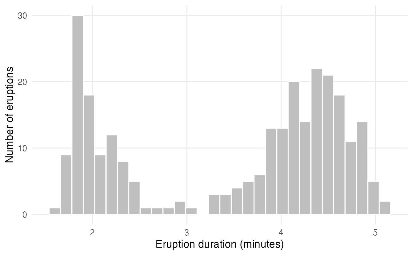

Figure 1: Durations of 272 eruptions of Old Faithful: two humps, short and long.

A two-component Gaussian mixture says that each eruption is generated in two stages:

1. nature first picks a type: short with probability \(\pi_1\), long with probability \(\pi_2 = 1 - \pi_1\);
2. then it draws the duration from a normal distribution with the mean \(\mu_g\) and standard deviation \(\sigma_g\) of that type.

So the density of a duration \(x\) is a weighted sum of two bell curves:

\[ f(x) = \pi_1\, \phi(x \mid \mu_1, \sigma_1) + \pi_2\, \phi(x \mid \mu_2, \sigma_2), \]

where \(\phi(x \mid \mu, \sigma)\) is the normal density (dnorm(x, mu, sigma) in R). The mixing proportions \(\pi_g\) are the cluster sizes in the population. We never observe the type, only the duration: the type is a latent (hidden) variable.

3. Fitting a mixture: the EM algorithm

If we knew the type of every eruption, fitting would be easy: compute the proportion, mean and SD of each type. If we knew the parameters, we could compute for each eruption the probability of each type. The EM algorithm (expectation–maximisation) alternates these two easy steps:

• E-step — with the current parameters, compute for every observation \(i\) the responsibility \(\tau_{ig}\): the probability that it belongs to component \(g\), given its value.
• M-step — re-estimate proportions, means and SDs as weighted averages, each observation counting for component \(g\) with weight \(\tau_{ig}\).

This is like k-means with soft assignments: instead of putting each point entirely in one cluster, EM splits it according to the probabilities. Here is a complete version for one variable:

em_1d <- function(x, mu, sigma, prop, max_iter = 500, tol = 1e-8) {
  loglik <- numeric(0)
  for (it in seq_len(max_iter)) {
    # E-step: weighted densities and responsibilities tau[i, g]
    dens <- sapply(seq_along(mu), \(g) prop[g] * dnorm(x, mu[g], sigma[g]))
    loglik[it] <- sum(log(rowSums(dens)))
    tau <- dens / rowSums(dens)
    # M-step: weighted proportions, means and standard deviations
    n_g   <- colSums(tau)
    prop  <- n_g / length(x)
    mu    <- colSums(tau * x) / n_g
    sigma <- sqrt(colSums(tau * outer(x, mu, "-")^2) / n_g)
    if (it > 1 && loglik[it] - loglik[it - 1] < tol) break
  }
  list(mu = mu, sigma = sigma, prop = prop, tau = tau, loglik = loglik)
}

We start from a rough guess — means 2 and 4, SDs 1, equal proportions — and let EM do the rest.

em <- em_1d(faithful$eruptions, mu = c(2, 4), sigma = c(1, 1),
            prop = c(0.5, 0.5))
round(c(prop = em$prop, mu = em$mu, sigma = em$sigma), 3)

#>  prop1  prop2    mu1    mu2 sigma1 sigma2 
#>  0.348  0.652  2.019  4.273  0.236  0.437

length(em$loglik)

#> [1] 25

round(em$loglik[c(1:4, length(em$loglik))], 2)

#> [1] -431.7 -372.5 -311.4 -282.5 -276.4

TipHow to read this output

• About 35% of eruptions are short, with mean 2.02 min and SD 0.24; the long ones have mean 4.27 min and a larger SD, 0.44.
• EM converged in 25 iterations. The log-likelihood (how probable the data are under the current parameters) increased at every iteration — this is guaranteed for EM — from -431.7 to -276.36.

curves <- tibble(x = seq(1.2, 5.6, length.out = 400)) |>
  mutate(
    short   = em$prop[1] * dnorm(x, em$mu[1], em$sigma[1]),
    long    = em$prop[2] * dnorm(x, em$mu[2], em$sigma[2]),
    mixture = short + long
  ) |>
  pivot_longer(-x, names_to = "curve", values_to = "density")

ggplot(faithful, aes(eruptions)) +
  geom_histogram(aes(y = after_stat(density)), bins = 30,
                 fill = "grey80", colour = "white") +
  geom_line(data = curves, aes(x, density, colour = curve,
                               linetype = curve), linewidth = 1) +
  scale_linetype_manual(values = c(long = 2, mixture = 1, short = 2)) +
  labs(x = "Eruption duration (minutes)", y = "Density",
       colour = NULL, linetype = NULL)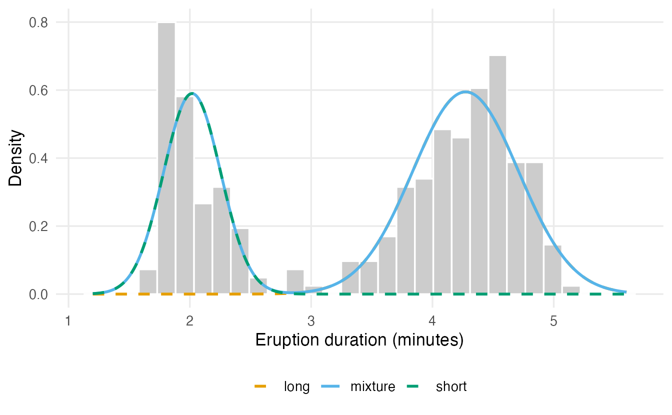

Figure 2: The fitted two-component mixture. Dashed: each component, weighted by its proportion; solid: their sum, the mixture density.

Soft assignments

The responsibilities are the soft assignment of each eruption. The hard cluster is the component with the largest responsibility, and \(1 - \max_g \tau_{ig}\) is the uncertainty:

cl_em  <- max.col(em$tau)
unc_em <- 1 - apply(em$tau, 1, max)
table(cl_em)

#> cl_em
#>   1   2 
#>  95 177

faithful |>
  mutate(p_short = round(em$tau[, 1], 3), uncertainty = round(unc_em, 3)) |>
  arrange(desc(uncertainty)) |>
  head(4)

#>   eruptions waiting p_short uncertainty
#> 1     2.800      56   0.544       0.456
#> 2     2.883      55   0.157       0.157
#> 3     2.900      63   0.112       0.112
#> 4     2.633      65   0.974       0.026

Almost all eruptions are classified with near certainty; only 3 have an uncertainty above 0.1. They lie in the valley between the two humps, where both components are plausible.

NoteGoing deeper: the EM equations and why the likelihood increases

With \(G\) components and parameters \(\theta = (\pi_g, \mu_g, \sigma_g)_{g=1}^G\), the log-likelihood is

\[ \ell(\theta) = \sum_{i=1}^n \log \sum_{g=1}^G \pi_g\, \phi(x_i \mid \mu_g, \sigma_g). \]

The log of a sum is hard to maximise directly. EM introduces the latent labels \(z_i\) and iterates:

E-step. \(\displaystyle \tau_{ig} = P(z_i = g \mid x_i; \theta^{(t)}) = \frac{\pi_g \phi(x_i \mid \mu_g, \sigma_g)}{\sum_h \pi_h \phi(x_i \mid \mu_h, \sigma_h)}\).

M-step. With \(n_g = \sum_i \tau_{ig}\): \[ \pi_g = \frac{n_g}{n}, \qquad \mu_g = \frac{1}{n_g}\sum_i \tau_{ig}\, x_i, \qquad \sigma_g^2 = \frac{1}{n_g}\sum_i \tau_{ig}\,(x_i - \mu_g)^2 . \]

These are exactly the lines of em_1d(). Each iteration maximises a lower bound of \(\ell\) that touches \(\ell\) at the current parameters, so \(\ell(\theta^{(t+1)}) \ge \ell(\theta^{(t)})\). Like k-means, EM converges to a local maximum, so the starting values matter. A direct numerical check: maximising \(\ell\) with a general-purpose optimiser reaches the same value.

x  <- faithful$eruptions
nll <- function(p) {      # p = (logit pi1, mu1, mu2, log s1, log s2)
  -sum(log(plogis(p[1]) * dnorm(x, p[2], exp(p[4])) +
           (1 - plogis(p[1])) * dnorm(x, p[3], exp(p[5]))))
}
opt <- optim(c(0, 2, 4, 0, 0), nll, method = "BFGS")
c(optim = -opt$value, em = tail(em$loglik, 1))

#>  optim     em 
#> -276.4 -276.4

4. The same model with mclust

The mclust package (Scrucca, Fop, Murphy & Raftery, 2016) fits Gaussian mixtures by EM, chooses good starting values, and compares many models. In one dimension there are two covariance models: "E" (equal variance in all components) and "V" (variable variances). Our em_1d() fit is the "V" model with \(G = 2\):

fit_v2 <- Mclust(faithful$eruptions, G = 2, modelNames = "V")
rbind(
  mclust = c(fit_v2$parameters$pro, fit_v2$parameters$mean,
             sqrt(fit_v2$parameters$variance$sigmasq)),
  em_1d  = c(em$prop, em$mu, em$sigma)
) |> round(3)

#>                        1     2            
#> mclust 0.349 0.651 2.019 4.274 0.236 0.437
#> em_1d  0.348 0.652 2.019 4.273 0.236 0.437

The estimates agree (up to the order of the components and tiny numerical differences). Now let mclust choose the number of components and the model by BIC:

bic_f <- mclustBIC(faithful$eruptions, G = 1:6)
summary(bic_f)

#> Best BIC values:
#>             V,4      V,2      V,3
#> BIC      -576.7 -580.752 -580.804
#> BIC diff    0.0   -4.092   -4.144

plot(bic_f)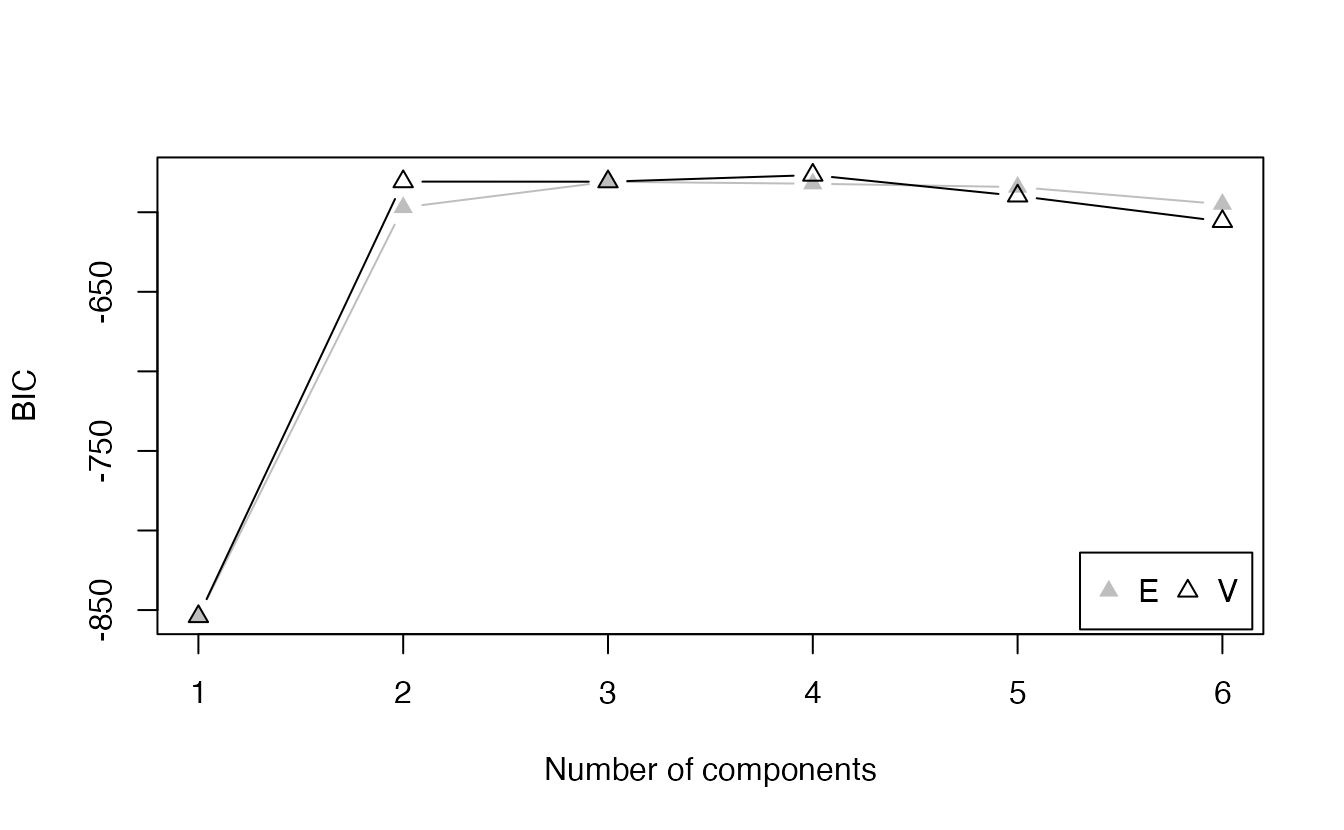

Figure 3: BIC of one-dimensional mixtures with 1 to 6 components, for equal (E) and variable (V) variances. In mclust the best model has the highest BIC.

ImportantIn mclust, higher BIC is better

Many textbooks define \(\text{BIC} = -2\log L + m \log n\) (lower is better). mclust uses the opposite sign: \[ \text{BIC} = 2 \log L - m \log n , \] where \(m\) is the number of free parameters and \(n\) the sample size. The first term rewards fit, the second penalises complexity. Choose the model with the largest BIC. A difference of less than about 2 is usually considered weak evidence; above 10, strong.

Let us check the formula with our own fit. With one component the model has \(m = 2\) parameters (mean, variance); with two “V” components, \(m = 5\) (two means, two variances, one free proportion):

x <- faithful$eruptions
n <- length(x)
s1 <- sqrt(mean((x - mean(x))^2))            # maximum likelihood SD
c(G1 = 2 * sum(dnorm(x, mean(x), s1, log = TRUE)) - 2 * log(n),
  G2 = 2 * tail(em$loglik, 1) - 5 * log(n))

#>     G1     G2 
#> -854.0 -580.7

c(mclust_G1 = bic_f[1, "V"], mclust_G2 = bic_f[2, "V"])

#> mclust_G1 mclust_G2 
#>    -854.0    -580.8

Two components are far better than one. summary(bic_f) lists the top three models; if a model with more than two components wins, look at the BIC differences before concluding that there are more than two types of eruption: extra components often just describe a skewed or flat-topped hump more flexibly.

5. More dimensions: covariance models

With \(p\) variables, each component \(g\) has a mean vector \(\mu_g\) and a covariance matrix \(\Sigma_g\), which describes the shape of its cloud of points: a sphere, an axis-aligned ellipse, or a tilted ellipse. mclust writes each covariance as

\[ \Sigma_g = \lambda_g\, D_g A_g D_g^\top , \]

with three geometric ingredients:

• volume \(\lambda_g\) — how big the cloud is;
• shape \(A_g\) — how elongated it is (a diagonal matrix of relative axis lengths);
• orientation \(D_g\) — in which direction it points.

Each ingredient can be Equal across components, Variable, or (for shape and orientation) the Identity. The three-letter model names spell volume–shape–orientation:

Model	Volume	Shape	Orientation	Clusters look like
EII	equal	identity	—	spheres of the same size (closest to k-means)
VII	variable	identity	—	spheres of different sizes
EEI	equal	equal	axes	identical axis-aligned ellipses
VVI	variable	variable	axes	different axis-aligned ellipses
EEE	equal	equal	equal	identical tilted ellipses (one common covariance)
VEV, EVV, …	mixed	mixed	variable	intermediate constraints
VVV	variable	variable	variable	each cluster its own covariance (most flexible)

mclust fits 14 such models (?mclustModelNames lists them all). Simple models have few parameters and are stable; VVV has \(G\,p(p+1)/2\) covariance parameters, which becomes a lot with many variables and few observations. BIC weighs fit against this cost.

NoteGoing deeper: k-means as a special case

Take a mixture with equal proportions and model EII (\(\Sigma_g = \lambda I\) for all \(g\)). If we replace the soft E-step by a hard one (assign each point to the component with the highest responsibility) and let \(\lambda \to 0\), the responsibilities become 0/1 according to the nearest mean and the M-step computes cluster means: this is exactly k-means. So k-means implicitly assumes spherical clusters of equal size and spread. Mixture models relax every part of that assumption.

6. Penguins: does a mixture find the species?

We use the same four standardised measurements as in the previous lessons. (Standardising is not strictly required for the most flexible models, but it puts the variables on comparable scales, which matters for the simpler models such as EII and for the starting values.)

peng <- penguins |>
  select(species, bill_len, bill_dep, flipper_len, body_mass) |>
  na.omit()
peng_z <- scale(select(peng, -species))

fit_p <- Mclust(peng_z, G = 1:9)
summary(fit_p)

#> ---------------------------------------------------- 
#> Gaussian finite mixture model fitted by EM algorithm 
#> ---------------------------------------------------- 
#> 
#> Mclust VEE (ellipsoidal, equal shape and orientation) model with 4 components: 
#> 
#>  log-likelihood   n df   BIC   ICL
#>           -1155 342 32 -2497 -2536
#> 
#> Clustering table:
#>   1   2   3   4 
#> 154  66  57  65

TipHow to read this output

• The header names the selected model: here VEE with 4 components — that is, the covariance model and \(G\) with the highest BIC among all those fitted.
• log-likelihood, n, df (number of parameters) and BIC are the ingredients of the formula above; ICL is a related criterion (section 9).
• The clustering table gives the size of each (hard) cluster.

plot(fit_p, what = "BIC")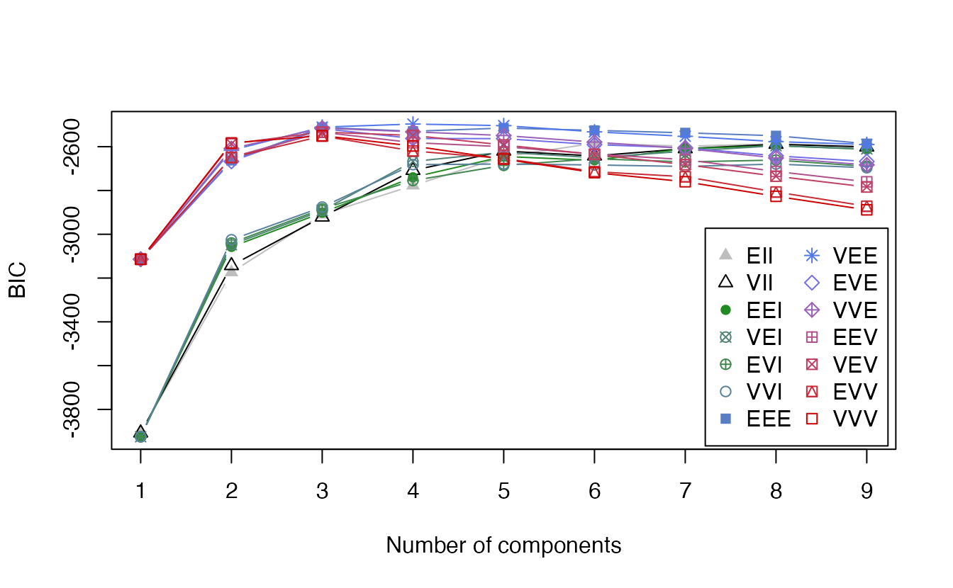

Figure 4: BIC for the 14 covariance models and 1 to 9 components on the penguin data. Higher is better.

table(cluster = fit_p$classification, species = peng$species)

#>        species
#> cluster Adelie Chinstrap Gentoo
#>       1    150         4      0
#>       2      0         0     66
#>       3      0         0     57
#>       4      1        64      0

fit_p3 <- Mclust(peng_z, G = 3)
set.seed(1)
km_p <- kmeans(peng_z, centers = 3, nstart = 25)
c(mclust_BIC_choice = adjustedRandIndex(fit_p$classification, peng$species),
  mclust_G3         = adjustedRandIndex(fit_p3$classification, peng$species),
  kmeans_k3         = adjustedRandIndex(km_p$cluster, peng$species))

#> mclust_BIC_choice         mclust_G3         kmeans_k3 
#>            0.8139            0.9605            0.7928

BIC chooses \(G =\) 4. With \(G = 3\), the mixture (model VEE) reaches an ARI with the species of 0.96, against 0.79 for k-means. Allowing elliptical, correlated clusters helps here: within a species, bill length, flipper length and body mass grow together, so each species forms a tilted ellipse rather than a sphere. Note also that the number of components preferred by BIC need not equal the number of species: BIC chooses the best density model, and a single species may be better described by more than one Gaussian (for instance, males and females).

7. Soft assignments and uncertainty

Mclust stores the responsibilities in $z (one column per cluster) and the uncertainty \(1 - \max_g \tau_{ig}\) in $uncertainty.

round(head(fit_p3$z), 3)

#>   [,1] [,2] [,3]
#> 1 1.00    0 0.00
#> 2 1.00    0 0.00
#> 3 0.99    0 0.01
#> 5 1.00    0 0.00
#> 6 1.00    0 0.00
#> 7 1.00    0 0.00

summary(fit_p3$uncertainty)

#>     Min.  1st Qu.   Median     Mean  3rd Qu.     Max. 
#> 0.00e+00 0.00e+00 2.50e-06 1.05e-02 2.34e-04 4.27e-01

peng |>
  mutate(cluster = fit_p3$classification,
         uncertainty = fit_p3$uncertainty) |>
  arrange(desc(uncertainty)) |>
  head(5)

#>     species bill_len bill_dep flipper_len body_mass cluster uncertainty
#> 1 Chinstrap     46.0     18.9         195      4150       1      0.4268
#> 2 Chinstrap     43.5     18.1         202      3400       3      0.3939
#> 3    Adelie     45.8     18.9         197      4150       1      0.3923
#> 4 Chinstrap     42.5     16.7         187      3350       1      0.3482
#> 5 Chinstrap     45.2     17.8         198      3950       3      0.3214

The most uncertain birds are the ones that sit between two clusters — often Adelie and Chinstrap penguins with intermediate measurements. A hard clustering method would assign them with apparent confidence; the mixture tells us honestly that it is not sure. A practical use: report the clusters for confidently assigned observations, and flag the uncertain ones (say, uncertainty > 0.2) for closer inspection.

8. Wholesale customers

Now the wholesale data, with the usual preprocessing.

wholesale <- read_csv(data_path("wholesale_customers.csv"),
                      show_col_types = FALSE)
spend_vars <- c("Fresh", "Milk", "Grocery", "Frozen",
                "Detergents_Paper", "Delicassen")

X <- wholesale |>
  select(all_of(spend_vars)) |>
  mutate(across(everything(), log1p)) |>
  scale()

fit_w <- Mclust(X, G = 1:9)
summary(fit_w)

#> ---------------------------------------------------- 
#> Gaussian finite mixture model fitted by EM algorithm 
#> ---------------------------------------------------- 
#> 
#> Mclust VVE (ellipsoidal, equal orientation) model with 5 components: 
#> 
#>  log-likelihood   n df   BIC   ICL
#>           -2823 440 79 -6126 -6247
#> 
#> Clustering table:
#>   1   2   3   4   5 
#>  51 101 155  81  52

summary(fit_w$BIC)

#> Best BIC values:
#>          VVE,5    VVE,3    VVE,6
#> BIC      -6126 -6155.13 -6186.58
#> BIC diff     0   -29.15   -60.61

plot(fit_w, what = "BIC")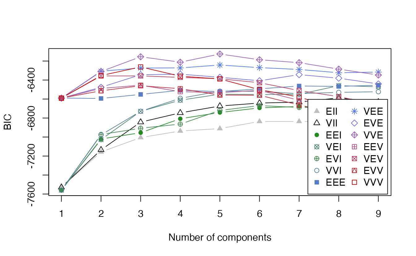

Figure 5: BIC by number of components and covariance model, wholesale data.

TipHow to read this output

• summary(fit_w) gives the chosen model (VVE, \(G =\) 5) and the cluster sizes.
• summary(fit_w$BIC) lists the three best models with their BIC differences from the best. If the runners-up are within a few BIC units and have a different \(G\), the data do not decide the number of clusters clearly — common with customer data.
• In the BIC plot, a curve that keeps rising slowly with \(G\) is a sign that the mixture is mainly describing a non-Gaussian shape of the data, not well-separated groups.

Comparison with k-means and with the sales channel

set.seed(123)
km_w <- kmeans(X, centers = fit_w$G, nstart = 50)
c(mclust_vs_kmeans  = adjustedRandIndex(fit_w$classification, km_w$cluster),
  mclust_vs_channel = adjustedRandIndex(fit_w$classification,
                                        wholesale$Channel),
  kmeans_vs_channel = adjustedRandIndex(km_w$cluster, wholesale$Channel))

#>  mclust_vs_kmeans mclust_vs_channel kmeans_vs_channel 
#>            0.3912            0.2629            0.2110

summary(fit_w$uncertainty)

#>    Min. 1st Qu.  Median    Mean 3rd Qu.    Max. 
#>  0.0000  0.0134  0.0457  0.1140  0.1610  0.6012

With the same number of clusters, the mixture and k-means agree with ARI 0.39. A clearly lower value than 1 means that the elliptical, unequal clusters of the mixture draw different boundaries from the spherical ones of k-means. Unlike k-means, the mixture also tells us that 96 clients (22%) have an uncertainty above 0.2.

pc <- prcomp(X)$x
tibble(PC1 = pc[, 1], PC2 = pc[, 2],
       cluster = factor(fit_w$classification),
       certainty = 1 - fit_w$uncertainty) |>
  ggplot(aes(PC1, PC2, colour = cluster, alpha = certainty)) +
  geom_point(size = 1.8) +
  scale_alpha(range = c(0.15, 1)) +
  labs(colour = "Cluster", alpha = "1 − uncertainty")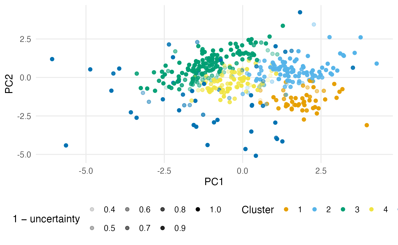

Figure 6: Mixture clusters on the first two principal components. Faint points are uncertain assignments.

Profiles in the original units

As always, describe the clusters with quantities a manager understands: median annual spending per category, plus the cluster size.

wholesale |>
  mutate(cluster = factor(fit_w$classification)) |>
  summarise(n = n(), across(all_of(spend_vars), median), .by = cluster) |>
  arrange(cluster)

#> # A tibble: 5 × 8
#>   cluster     n  Fresh  Milk Grocery Frozen Detergents_Paper Delicassen
#>   <fct>   <int>  <dbl> <dbl>   <dbl>  <dbl>            <dbl>      <dbl>
#> 1 1          51  1454   7845  13567   283             6830        716  
#> 2 2         101  7842   7243  11238  1389             4621       1625  
#> 3 3         155 14276   1786   2405  3383              325        933  
#> 4 4          81  5969   3218   3133   907              637        656  
#> 5 5          52  2270.  1572   3712.  892.5            174.5      284.5

table(cluster = fit_w$classification, channel = wholesale$Channel)

#>        channel
#> cluster   1   2
#>       1   7  44
#>       2  18  83
#>       3 149   6
#>       4  77   4
#>       5  47   5

The mixture means (fit_w$parameters$mean) are on the standardised log scale, so they are useful for comparing clusters but not for reporting. The medians above are in the original monetary units. The cross-table with Channel (1 = Horeca, 2 = Retail), which was not used for clustering, helps to name the clusters.

9. ICL: a criterion that prefers well-separated clusters

BIC selects the best model for the density of the data. If two heavily overlapping Gaussians describe a skewed cluster better than one, BIC will choose two — even though, as clusters, they are not separate. The integrated complete-data likelihood (ICL; Biernacki, Celeux & Govaert, 2000) adds a penalty for overlap: it is BIC minus a term that grows when the responsibilities are far from 0 and 1. ICL therefore tends to choose fewer, better-separated clusters.

icl_w <- mclustICL(X, G = 1:9)
summary(icl_w)

#> Best ICL values:
#>          VVE,3     VVE,5   VVE,4
#> ICL      -6244 -6246.878 -6331.4
#> ICL diff     0    -3.192   -87.7

If BIC and ICL agree, good. If ICL picks fewer components, the extra components chosen by BIC probably describe the shape of clusters rather than additional groups. Report which criterion you used and why.

WarningCommon pitfalls

1. Choosing the model with the smallest BIC. In mclust, BIC is defined so that higher is better.
2. Equating mixture components with groups. A non-Gaussian cluster (skewed, curved) may need several Gaussian components. Use ICL, look at the plots, and merge components if they describe one group.
3. Ignoring the uncertainty. Soft assignments are the main extra information a mixture provides; report how many observations are uncertain.
4. Too many parameters. VVV with many variables and few observations may be unstable or fail to fit; mclust then reports missing BIC values for those models. Simpler covariance models or dimension reduction help.
5. Describing clusters only by the fitted means on the transformed scale. Give medians (or means) in the original units.
6. Forgetting that EM finds a local optimum. mclust uses careful starting values, but different preprocessing or a different subsample can change the solution; check stability as in the introduction.

10. Check your understanding

NoteQ1. Two models have BIC −2540 and −2525 in mclust. Which is preferred, and how strongly?

The one with −2525: it is higher by 15, which by the usual scale is strong evidence.

NoteQ2. An observation has responsibilities (0.48, 0.47, 0.05). What are its hard cluster and its uncertainty, and what would you do with it?

Hard cluster 1 (the largest responsibility), uncertainty \(1 - 0.48 = 0.52\). It sits between clusters 1 and 2 and should not be treated as a typical member of either; flag it or report it as “between 1 and 2”.

NoteQ3. Which mclust covariance model corresponds most closely to the assumptions of k-means?

EII: spherical clusters with equal volume. k-means is its hard-assignment limit with equal proportions.

NoteQ4. Why can BIC choose four components when you believe there are two groups?

Because BIC chooses the best density model, not the best partition. If a group is skewed or has a non-elliptical shape, two Gaussians may describe it better than one. ICL, which penalises overlapping components, is more aligned with “clusters”.

11. Exercises

★ Exercise 1 — predict the responsibilities. Using the fitted parameters in em, an eruption of 3 minutes is closer to the short mean (about 2.0) than to the long mean (about 4.3). Predict which component it is assigned to, then compute its responsibilities with em$prop * dnorm(3, em$mu, em$sigma), normalised to sum to 1.

TipSolution

d <- em$prop * dnorm(3, em$mu, em$sigma)
round(d / sum(d), 3)        # about 0.012 (short) and 0.988 (long)

Surprisingly, it goes to the long component with probability about 0.99. The short component is narrow (SD about 0.24), so 3 minutes is about 4 of its SDs away; the long component is wider (SD about 0.44), and 3 minutes is less than 3 of its SDs away. A mixture measures distance in units of each cluster’s own spread; k-means, which uses raw distance to the means, would assign this eruption to the short cluster.

★ Exercise 2 — debug. A student writes: “I fitted Mclust() and kept the model with the smallest BIC, which was EII with one component.” What went wrong?

TipSolution

In mclust, BIC \(= 2\log L - m\log n\), so larger is better. The student picked the worst model. The fitted object already contains the best one (fit$modelName, fit$G), and summary(fit$BIC) lists the top three.

★★ Exercise 3 — EM and starting values. Run em_1d() on faithful$eruptions starting from mu = c(3.5, 3.5), sigma = c(1, 1), prop = c(0.5, 0.5). What do you get, and why? Then start from mu = c(1.5, 5.5), sigma = c(0.1, 0.1).

TipSolution

em_sym <- em_1d(faithful$eruptions, mu = c(3.5, 3.5), sigma = c(1, 1),
                prop = c(0.5, 0.5))
em_sym[c("mu", "sigma", "prop")]

With identical starting components, both get the same responsibilities (0.5 each) for every observation, so the M-step makes them identical again: the algorithm stays stuck on a symmetric solution where both components equal the overall mean (about 3.49) and SD (about 1.14). EM never breaks a perfect symmetry on its own. From the second, asymmetric start, EM reaches the same solution as before (log-likelihood about −276.4): starting values matter, but a reasonable asymmetric start is usually enough in simple problems.

★★ Exercise 4 — interpret. A Gaussian mixture on 1,000 customers gives: model VEV, \(G = 4\); sizes 410, 290, 220, 80; 170 customers with uncertainty > 0.2; ICL selects \(G = 3\). Write three sentences for a report.

TipSolution

The best density model by BIC has four elliptical clusters with different volumes and orientations but a common shape. About 17% of customers are assigned with substantial uncertainty, so the boundaries between clusters are fuzzy. Since ICL prefers three clusters, two of the four components probably overlap and may describe a single, non-Gaussian group; I would examine which two, and present the three-group solution unless the fourth component has a clear and useful interpretation.

★★★ Exercise 5 — mini-analysis: elongated clusters. Recreate the elongated bands from the k-means lesson, section 8 (set.seed(6), two horizontal bands). Fit Mclust(..., G = 2) and k-means with \(k = 2\), and compare both with the truth using the ARI. Which covariance model does Mclust select, and why does it succeed?

TipSolution

set.seed(6)
elongated <- tibble(
  x = c(rnorm(150, 0, 3), rnorm(150, 0, 3)),
  y = c(rnorm(150, 0, 0.3), rnorm(150, 2, 0.3)),
  truth = rep(1:2, each = 150)
)
xy <- elongated[, c("x", "y")]
fit_el <- Mclust(xy, G = 2)
set.seed(1)
km_el <- kmeans(xy, centers = 2, nstart = 25)
fit_el$modelName
c(mclust = adjustedRandIndex(fit_el$classification, elongated$truth),
  kmeans = adjustedRandIndex(km_el$cluster, elongated$truth))

k-means has ARI near 0 (it cuts the bands vertically); the mixture should be close to 1. The selected model typically has elongated, axis-aligned components (a diagonal model such as EEI): each band is a normal cloud with large variance in \(x\) and small variance in \(y\), which a covariance matrix can represent and a sphere cannot.

★★★ Exercise 6 — profile and name. For the wholesale mixture fit_w, compute the mean responsibility of each cluster within each Channel (aggregate(fit_w$z, list(channel = wholesale$Channel), mean)) and the median spending per cluster. Give each cluster a short name and say which one is the least clearly defined.

TipSolution

aggregate(fit_w$z, list(channel = wholesale$Channel), mean)
wholesale |>
  mutate(cluster = fit_w$classification, unc = fit_w$uncertainty) |>
  summarise(n = n(), mean_uncertainty = mean(unc),
            across(all_of(spend_vars), median), .by = cluster)

Names follow from the profiles: clusters with high Grocery, Milk and Detergents_Paper and many Retail clients (“shop-like”), clusters with high Fresh and Frozen and many Horeca clients (“restaurant-like”), and possibly a small cluster with low spending overall. The least clearly defined cluster is the one with the highest mean uncertainty — its members are often between two other clusters. Your exact names depend on the solution selected by BIC.

Summary

Task	Code	Remember
Fit a mixture (BIC choice)	Mclust(x, G = 1:9)	scale first for multivariate data
Fix \(G\) / model	Mclust(x, G = 3, modelNames = "VVV")	1-D models: "E", "V"
BIC table and plot	mclustBIC(x), summary(fit$BIC), plot(fit, what = "BIC")	higher is better
Chosen model	fit$modelName, fit$G	volume–shape–orientation letters
Hard / soft assignment	fit$classification, fit$z	rows of z sum to 1
Uncertainty	fit$uncertainty	\(1 - \max_g \tau_{ig}\)
Parameters	fit$parameters$pro, $mean, $variance	on the scale of the fitted data
Separation-oriented choice	mclustICL(x)	fewer, better-separated clusters
Compare partitions	adjustedRandIndex(a, b)	e.g. with k-means

• A Gaussian mixture models the data as a weighted sum of normal distributions; each component is a cluster.
• EM alternates soft assignment (E) and weighted estimation (M); it increases the likelihood and reaches a local maximum.
• Covariance models (EII … VVV) control the volume, shape and orientation of clusters; BIC (higher is better) chooses the model and \(G\), ICL favours separated clusters.
• Soft assignments and uncertainty show which observations are ambiguous — information that k-means cannot give.
• Profile the clusters in original units and check them against external information when it exists.

NoteFurther reading

• Scrucca, L., Fop, M., Murphy, T. B. & Raftery, A. E. (2016). mclust 5: clustering, classification and density estimation using Gaussian finite mixture models. The R Journal, 8(1), 289–317. https://journal.r-project.org/archive/2016/RJ-2016-021/
• Documentation and vignette of the mclust package, https://cran.r-project.org/package=mclust
• James, Witten, Hastie & Tibshirani, An Introduction to Statistical Learning (2e), chapter 12, https://www.statlearning.com