library(dplyr)
library(ggplot2)Non-parametric tests
Rank-based tests, rank correlation and permutation tests — and when you actually need them
Learn what rank-based tests do, run the Wilcoxon, Mann–Whitney, Kruskal–Wallis and Spearman tests in R, understand what hypotheses they really test, and use permutation tests as a flexible alternative.
NoteLearning objectives
By the end of this lesson you will be able to:
- explain what “non-parametric” and “rank-based” mean;
- run the Wilcoxon signed-rank, Wilcoxon rank-sum (Mann–Whitney) and Kruskal–Wallis tests and follow up with adjusted pairwise comparisons;
- state what these tests actually test (and why it is not simply “the medians”);
- compare Pearson and Spearman correlation tests with
cor.test(); - write a permutation test for any statistic, and decide when a non-parametric method is really needed.
1. Why another family of tests?
The t-test of t-tests compares means and uses the t distribution as its null distribution. That works well when samples are large or the data are roughly normal. It can work poorly when:
- samples are small and the data are clearly skewed or contain outliers: one extreme value can drag the mean and inflate the standard deviation;
- the data are ordinal — scores such as “1 = poor … 5 = excellent”, where differences between categories are not equal distances, so a mean is hard to interpret.
Non-parametric methods make fewer assumptions about the shape of the distribution (they do not assume it belongs to a family described by a few parameters, such as the normal). The classical ones work on ranks instead of the raw values.
2. From values to ranks
x <- c(3.1, 10, 2.5, 2.5, 7, 250)
rank(x)
#> [1] 3.0 5.0 1.5 1.5 4.0 6.0The smallest value gets rank 1, the next rank 2, and so on; tied values share the average of their ranks (the two 2.5’s get 1.5 each). Notice the last value: whether it is 250 or 11, its rank is 6. Ranks are insensitive to how extreme an outlier is — this is where the robustness of rank tests comes from. The price is that some information about distances is thrown away.
3. Wilcoxon signed-rank test (one sample or paired)
The sleep data (used in t-tests) give the extra hours of sleep for the same 10 patients under two drugs. The paired t-test works on the differences; the signed-rank test ranks the absolute differences and then compares the sum of ranks of the positive and the negative differences.
drug1 <- sleep$extra[sleep$group == 1]
drug2 <- sleep$extra[sleep$group == 2]

wsr <- wilcox.test(drug2, drug1, paired = TRUE)
wsr
#>
#> Wilcoxon signed rank exact test
#>
#> data: drug2 and drug1
#> V = 54, p-value = 0.004
#> alternative hypothesis: true location shift is not equal to 0t.test(drug2, drug1, paired = TRUE)$p.value#> [1] 0.002833
TipHow to read this output
- V is the sum of the ranks of the positive differences (54). Here 9 of the 10 patients slept more with drug 2 and one had no change, so the rank sum comes entirely from positive differences. (How zero differences are handled varies between methods; see
?wilcox.test.) - p-value: 0.0039. If the differences were symmetric around 0, a rank sum this lopsided would be rare.
- “true location shift is not equal to 0”: \(H_0\) is that the differences are symmetric around 0.
- The paired t-test reaches the same conclusion. With clean data the two tests usually agree.
For a single sample, wilcox.test(x, mu = m0) tests whether the distribution is symmetric around m0.
4. Wilcoxon rank-sum = Mann–Whitney test (two independent groups)
The chickwts data give the weight of chicks fed different diets. Compare horsebean with linseed:
chicks2 <- chickwts |>
  filter(feed %in% c("horsebean", "linseed")) |>
  droplevels()

tapply(chicks2$weight, chicks2$feed, median)
#> horsebean linseed
#> 151.5 221.0The rank-sum test pools the two groups, ranks all observations together and checks whether one group’s ranks are systematically higher. The same test is known as the Mann–Whitney U test.
mw <- wilcox.test(weight ~ feed, data = chicks2, conf.int = TRUE)
mw
#>
#> Wilcoxon rank sum exact test
#>
#> data: weight by feed
#> W = 20, p-value = 0.007
#> alternative hypothesis: true location shift is not equal to 0
#> 96 percent confidence interval:
#> -105 -12
#> sample estimates:
#> difference in location
#> -60.5
TipHow to read this output
- W = 20 counts, over all 120 horsebean–linseed pairs, how many times the horsebean chick is heavier. So \(W / (n_1 n_2)\) = 0.17 estimates \(P(\text{horsebean} > \text{linseed})\). Under \(H_0\) this probability would be 0.5.
- p-value 0.0071: horsebean chicks tend to be lighter.
- difference in location (-60.5 g) with its CI (for exact tests R reports the achievable confidence level, which can be slightly above 95%): the Hodges–Lehmann estimate, the median of all pairwise differences. It is a sensible summary of the shift if the two distributions have the same shape.
What does the rank-sum test really test?
It is often said that the Mann–Whitney test “compares medians”. That is only true under an extra assumption: that the two distributions have the same shape and differ only by a shift. In general, it tests whether one group tends to produce larger values than the other, i.e. whether \(P(X > Y) \neq 0.5\) (stochastic dominance).
A simulation makes the difference visible. Below, both groups have exactly the same median (0), but one is skewed to the right and the other to the left:
set.seed(10)
reject <- replicate(2000, {
  x <- rexp(100) - log(2)       # median 0, long right tail
  y <- -(rexp(100) - log(2))    # median 0, long left tail
  wilcox.test(x, y)$p.value < 0.05
})
mean(reject)
#> [1] 0.6675The test rejects in 67% of the samples, although the medians are equal. It is not wrong: \(X\) really does tend to be larger than \(Y\). It just does not answer a question about medians. Say “the values in group A tend to be larger”, not “the medians differ”, unless the shapes look similar.
NoteGoing deeper: the statistics
- Signed-rank: rank \(|d_i|\) for the non-zero differences; \(V = \sum_{d_i > 0} \text{rank}(|d_i|)\). Under \(H_0\) each sign is + or − with probability 1/2, so the null distribution of \(V\) can be enumerated exactly (small \(n\)) or approximated by a normal.
- Rank-sum: \(W = \sum_{i}\sum_{j} \mathbf 1(x_i > y_j)\) (ties count 1/2). This is R’s \(W\); it equals the sum of the ranks of the first sample minus \(n_1(n_1+1)/2\). Under \(H_0\) (same distribution), \(E[W] = n_1 n_2 / 2\).
- Efficiency: for normal data, rank tests lose little: their asymptotic relative efficiency compared with the t-test is \(3/\pi \approx 0.955\). For heavy-tailed data they can be far more powerful than the t-test.
5. Kruskal–Wallis test (three or more groups)
The rank-based version of one-way ANOVA (see ANOVA): are all groups drawn from the same distribution?
ggplot(chickwts, aes(reorder(feed, weight, FUN = median), weight)) +
  geom_boxplot(outlier.shape = NA) +
  geom_jitter(width = 0.15, alpha = 0.5) +
  labs(x = "Feed (ordered by median weight)", y = "Weight (g)")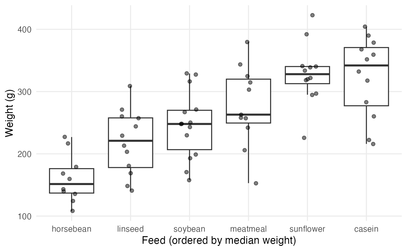
kw <- kruskal.test(weight ~ feed, data = chickwts)
kw
#>
#> Kruskal-Wallis rank sum test
#>
#> data: weight by feed
#> Kruskal-Wallis chi-squared = 37, df = 5, p-value = 5e-07The p-value (5.1e-07) says that at least one feed differs from the others. To see which pairs differ, use pairwise rank-sum tests with a multiple-testing adjustment (see Hypothesis testing):
pairwise.wilcox.test(chickwts$weight, chickwts$feed,
                     p.adjust.method = "holm", exact = FALSE)
#>
#> Pairwise comparisons using Wilcoxon rank sum test with continuity correction
#>
#> data: chickwts$weight and chickwts$feed
#>
#> casein horsebean linseed meatmeal soybean
#> horsebean 0.003 - - - -
#> linseed 0.012 0.064 - - -
#> meatmeal 0.362 0.009 0.218 - -
#> soybean 0.047 0.009 0.710 0.710 -
#> sunflower 1.000 0.002 0.003 0.347 0.014
#>
#> P value adjustment method: holm
TipHow to read this output
Each cell is a Holm-adjusted p-value for one pair of feeds. For example, horsebean differs from casein and sunflower (adjusted p well below 0.01), while casein and sunflower are indistinguishable. exact = FALSE uses the normal approximation, which avoids warnings when there are ties.
6. Correlation: Pearson and Spearman side by side
cor.test() tests \(H_0\): “no correlation”. The Pearson correlation measures linear association; the Spearman correlation is the Pearson correlation of the ranks, so it measures monotonic association (one variable tends to increase with the other, not necessarily in a straight line). See Correlation for the descriptive side.
pear <- cor.test(~ Ozone + Temp, data = airquality)
spear <- cor.test(~ Ozone + Temp, data = airquality,
                  method = "spearman", exact = FALSE)
c(pearson = unname(pear$estimate), spearman = unname(spear$estimate))
#> pearson spearman
#> 0.6984 0.7740c(pearson = pear$p.value, spearman = spear$p.value)#> pearson spearman
#> 2.932e-18 2.248e-24pear$conf.int#> [1] 0.5913 0.7812
#> attr(,"conf.level")
#> [1] 0.95Both indicate a strong positive association between temperature and ozone. Spearman’s \(\rho\) (0.77) is a bit higher than Pearson’s \(r\) (0.7) because the relationship curves upwards: it is monotonic but not linear. Only the Pearson test provides a confidence interval in cor.test().
The difference is dramatic when there is an outlier:
set.seed(4)
x <- 1:20
y <- x + rnorm(20, sd = 3)
y[20] <- -40                      # one wild value
c(pearson  = cor(x, y),
  spearman = cor(x, y, method = "spearman"))
#> pearson spearman
#> 0.04455 0.63759A single point destroys the Pearson correlation (it falls to 0.04), while Spearman’s (\(\rho =\) 0.64) still sees the clear increasing trend in the other 19 points. Always plot before you correlate.
7. Permutation tests: a flexible alternative
The permutation test of Hypothesis testing works with any statistic you choose. Suppose you really care about the difference in medians between horsebean and linseed chicks:
med_diff <- function(y, g) {
  m <- tapply(y, g, median)
  unname(m["linseed"] - m["horsebean"])
}
obs <- med_diff(chicks2$weight, chicks2$feed)

set.seed(1)
perm <- replicate(10000, med_diff(chicks2$weight, sample(chicks2$feed)))
p_perm <- mean(abs(perm) >= abs(obs))
c(observed = obs, p_value = p_perm)
#> observed p_value
#> 69.5000 0.0228The observed difference in medians is 69.5 g, and only 2.3% of the shuffled datasets produce one at least as large. The recipe is always the same: choose a statistic → shuffle under \(H_0\) → compare. It works for medians, trimmed means, ratios of variances, correlations, and more. Two requirements: under \(H_0\) the shuffled labels must be exchangeable (for example, independent units), and the shuffle must respect the design (for paired data, swap the values within each pair, rather than shuffling freely).
8. When to use what
| Situation | Parametric | Rank-based | Notes |
|---|---|---|---|
| One sample or paired differences | t.test(x, mu = ), t.test(..., paired = TRUE) |
wilcox.test(x, mu = ), wilcox.test(..., paired = TRUE) |
Signed-rank assumes symmetric differences |
| Two independent groups | t.test(y ~ g) (Welch) |
wilcox.test(y ~ g) |
Rank-sum tests \(P(X > Y) = 0.5\) |
| Three or more groups | aov(), oneway.test() |
kruskal.test() + pairwise.wilcox.test() |
See ANOVA |
| Association of two numeric variables | cor.test() (Pearson) |
cor.test(method = "spearman") |
Spearman: monotonic, robust to outliers |
| Any statistic, any design | — | Permutation test | Shuffle according to the design |
“My data aren’t normal” is not automatically a reason to switch
- With moderate or large samples, the t-test is robust: it is about the sampling distribution of the mean, which the Central Limit Theorem makes approximately normal (see Sampling distributions). Welch’s test also handles unequal variances.
- The tests answer different questions. The t-test is about means; the rank-sum test is about \(P(X > Y)\). If the mean is what matters (total cost, total yield), a rank test answers the wrong question.
- A formal normality test is a poor guide: with small samples it rarely detects non-normality, with large ones it flags harmless deviations. Look at plots and think about the data.
- Other options exist: a transformation (for example, the logarithm for right-skewed positive data), a bootstrap CI (Bootstrap), or a permutation test of the mean.
- Rank tests are a good choice for small samples with outliers or strong skew, for ordinal data, and when “tends to be larger” is the natural question.
WarningCommon pitfalls
- Saying “the medians differ” after a Mann–Whitney test. That is only justified if the distributions have similar shapes.
- Thinking non-parametric means assumption-free. Rank tests still assume independent observations; the signed-rank test assumes symmetric differences.
- Switching tests after seeing which one gives the smaller p-value. Choose the test from the question and the design, before the analysis.
- Using the rank-sum test on paired data (or the signed-rank test on independent groups). As with t-tests, the design decides.
- Forgetting the multiple-comparison adjustment after a significant Kruskal–Wallis test.
- Reporting only a p-value. Report an effect too: the Hodges–Lehmann shift with its CI, \(P(X > Y)\), or Spearman’s \(\rho\).
9. Check your understanding
10. Exercises
Interactive (run in your browser)
★ Exercise 1 — two independent groups. Compare mpg between automatic (am == 0) and manual (am == 1) cars in mtcars with a rank-sum test, and with a Welch t-test. Do they agree?
The formula is outcome ~ group, as in t.test().
wilcox.test(mpg ~ am, data = mtcars)Both tests find a clear difference (p about 0.001 for both the rank-sum test and Welch): manual cars tend to have higher mpg. With clear effects and reasonably shaped data, the two approaches agree.
★★ Exercise 2 — Kruskal–Wallis and follow-up. The InsectSprays data give insect counts on plots treated with six sprays (A–F). Counts are skewed and the variances differ a lot between sprays. Run a Kruskal–Wallis test and the Holm-adjusted pairwise comparisons. Which sprays seem most effective (lowest counts)?
The outcome is count and the group is spray; the adjustment method is "holm".
kruskal.test(count ~ spray, data = InsectSprays)
pairwise.wilcox.test(InsectSprays$count, InsectSprays$spray,
                     p.adjust.method = "holm", exact = FALSE)
The Kruskal–Wallis test is highly significant. Sprays C, D and E have the lowest medians, and each of them differs from A, B and F (adjusted p < 0.001). Among C, D and E, only C vs D reaches significance (about 0.016).
★★ Exercise 3 — an outlier and two correlations. Run the code and compare the Pearson and Spearman tests. Then remove the outlier (x[-20], y[-20]) and repeat the Pearson test. What changes?
Use method = "spearman", and -20 to drop the 20th element.
cor.test(x, y)$p.value                        # about 0.85
cor.test(x, y, method = "spearman")$p.value   # about 0.003
cor.test(x[-20], y[-20])$estimate             # about 0.9
With the outlier, Pearson sees no association; Spearman detects the trend. Without the outlier, Pearson’s r is high again. Never delete points just to obtain a result — but always investigate them: is it a data-entry error, or a real and interesting observation?
Practice on your own computer
★★★ Exercise 4 — a permutation test for paired data. For the sleep data, write a permutation test of the mean paired difference (drug 2 − drug 1). Under \(H_0\) each difference is equally likely to be positive or negative, so randomly flip the signs of the differences instead of shuffling labels. Compare with the paired t-test.
TipSolution
d <- sleep$extra[sleep$group == 2] - sleep$extra[sleep$group == 1]
obs <- mean(d)

set.seed(1)
perm <- replicate(10000, {
  signs <- sample(c(-1, 1), length(d), replace = TRUE)
  mean(signs * d)
})
mean(abs(perm) >= abs(obs))
t.test(d)$p.value
The sign-flip p-value is close to the paired t-test p-value (both well below 0.01: about 0.004 and 0.003). Shuffling freely between the two groups would break the pairing — the permutation must follow the design.
★★ Exercise 5 — choose the test. For each situation, name a suitable test and say why. (a) Pain scores (0–10) for 12 patients before and after physiotherapy. (b) Income of 800 men and 800 women, very right-skewed; the question is about average income. (c) Satisfaction ratings (1–5) for four different help-desk teams.
TipSolution
- Paired ordinal data with small \(n\): Wilcoxon signed-rank (
paired = TRUE). (b) The question is about means and \(n\) is large: Welch t-test (the CLT applies); a bootstrap CI for the difference in means, or an analysis on the log scale (which compares geometric means), are good complements. A rank test would answer a different question. (c) Ordinal outcome, four independent groups: Kruskal–Wallis, followed by Holm-adjusted pairwise Wilcoxon tests.
Summary
| Test | R | Tests whether… |
|---|---|---|
| Signed-rank | wilcox.test(x, mu = ) / wilcox.test(a, b, paired = TRUE) |
(differences) are symmetric around the reference |
| Rank-sum / Mann–Whitney | wilcox.test(y ~ g, conf.int = TRUE) |
one group tends to give larger values (\(P(X>Y) \ne 0.5\)) |
| Kruskal–Wallis | kruskal.test(y ~ g) + pairwise.wilcox.test() |
all groups come from the same distribution |
| Pearson / Spearman | cor.test(x, y) / cor.test(x, y, method = "spearman") |
linear / monotonic association |
| Permutation | replicate() + sample() |
any statistic you choose is larger than chance would give |
- Rank tests replace values by ranks: robust to outliers, suitable for ordinal data.
- The rank-sum test is not a test of medians unless the shapes are equal.
- Spearman is Pearson on ranks: it captures monotonic trends and resists outliers.
- Permutation tests are flexible; shuffle in a way that respects the design.
- Non-normal data with a decent sample size do not automatically require a non-parametric test — think about the question first.