library(dplyr)
library(ggplot2)
library(forcats)
library(broom)Multiple regression
Several predictors, factors, interactions — and the diagnostics that keep you honest
Interpret coefficients ‘holding the other predictors constant’, use categorical predictors and interactions, detect multicollinearity and influential points, handle heteroscedasticity with robust standard errors, and report a model clearly.
NoteLearning objectives
By the end of this lesson you will be able to:
- fit a regression with several predictors and interpret each coefficient holding the others constant;
- include categorical predictors, read their dummy coding and change the reference level;
- fit and visualise an interaction between a numeric predictor and a factor;
- diagnose multicollinearity (VIF), influential points (leverage, Cook’s distance) and heteroscedasticity, and compute robust standard errors;
- show a model’s predictions with a partial effect plot and report the model in words.
1. Why more than one predictor?
At the end of Simple regression we found that the slope of body mass on flipper length is about 50 g/mm across all penguins, but only about 33 g/mm within Adelie penguins. Gentoo penguins have both longer flippers and larger bodies, so part of the overall slope is really a species difference.
With a single predictor, every other influence is mixed into its slope. Multiple regression puts several predictors in the same model, so that each coefficient describes the association of one predictor with the response after accounting for the others.
2. Two numeric predictors: “holding the others constant”
Fuel efficiency (mpg) in the mtcars data falls with car weight (wt, in 1000 lb). Heavier cars also tend to have more horsepower (hp): the correlation between wt and hp is 0.66.
m_wt <- lm(mpg ~ wt, data = mtcars)
m_wt_hp <- lm(mpg ~ wt + hp, data = mtcars)

coef(m_wt)
#> (Intercept) wt
#> 37.285 -5.344coef(m_wt_hp)#> (Intercept) wt hp
#> 37.22727 -3.87783 -0.03177The coefficient of wt drops from -5.34 to -3.88. They answer different questions:
- Simple model: cars that are 1000 lb heavier have, on average, 5.3 fewer mpg — partly because heavier cars also have more powerful engines.
- Multiple model: among cars with the same horsepower, those that are 1000 lb heavier have, on average, 3.9 fewer mpg.
“Holding horsepower constant” is a statistical adjustment, not an experiment. Nobody added weight to a car while keeping its engine fixed; the model compares cars that differ in weight but have similar horsepower.
summary(m_wt_hp)#>
#> Call:
#> lm(formula = mpg ~ wt + hp, data = mtcars)
#>
#> Residuals:
#> Min 1Q Median 3Q Max
#> -3.941 -1.600 -0.182 1.050 5.854
#>
#> Coefficients:
#> Estimate Std. Error t value Pr(>|t|)
#> (Intercept) 37.22727 1.59879 23.28 < 2e-16 ***
#> wt -3.87783 0.63273 -6.13 1.1e-06 ***
#> hp -0.03177 0.00903 -3.52 0.0015 **
#> ---
#> Signif. codes: 0 '***' 0.001 '**' 0.01 '*' 0.05 '.' 0.1 ' ' 1
#>
#> Residual standard error: 2.59 on 29 degrees of freedom
#> Multiple R-squared: 0.827, Adjusted R-squared: 0.815
#> F-statistic: 69.2 on 2 and 29 DF, p-value: 9.11e-12
TipHow to read this output
- Each row of the coefficient table tests \(H_0: \beta_j = 0\) given the other predictors in the model. Both
wtandhpadd information beyond the other. - Multiple R-squared is 0.83. Adding a predictor can never decrease R²; adjusted R² (0.81) penalises each extra parameter and is fairer for comparing models of different size (more in Model selection).
- The F-statistic now tests all slopes at once: \(H_0: \beta_{wt} = \beta_{hp} = 0\).
NoteGoing deeper: what “adjusting” means (Frisch–Waugh–Lovell)
In matrix form \(y = X\beta + \varepsilon\), and OLS gives \(\hat\beta = (X^\top X)^{-1} X^\top y\).
The coefficient of wt in the multiple model equals the slope obtained by (1) regressing mpg on hp and keeping the residuals, (2) regressing wt on hp and keeping the residuals, (3) regressing the first residuals on the second. In words: it is the association between the parts of mpg and wt that hp cannot explain.
e_mpg <- resid(lm(mpg ~ hp, data = mtcars))
e_wt  <- resid(lm(wt ~ hp, data = mtcars))
coef(lm(e_mpg ~ e_wt))["e_wt"]
#> e_wt
#> -3.878The same number as in m_wt_hp.
3. Categorical predictors and dummy coding
Now add species to the penguin model.
m_add <- lm(body_mass ~ flipper_len + species, data = penguins)
tidy(m_add)
#> # A tibble: 4 × 5
#> term estimate std.error statistic p.value
#> <chr> <dbl> <dbl> <dbl> <dbl>
#> 1 (Intercept) -4031. 584.2 -6.901 2.551e-11
#> 2 flipper_len 40.71 3.071 13.25 1.402e-32
#> 3 speciesChinstrap -206.5 57.73 -3.577 3.981e- 4
#> 4 speciesGentoo 266.8 95.26 2.801 5.392e- 3A factor with \(k\) levels enters the model as \(k - 1\) dummy variables (0/1 indicators). The first level, here Adelie, is the reference level and has no dummy of its own. We can see this in the model matrix, the numeric table that lm() actually uses:
model.matrix(m_add)[c("1", "161", "302"), ]#> (Intercept) flipper_len speciesChinstrap speciesGentoo
#> 1 1 181 0 0
#> 161 1 209 0 1
#> 302 1 197 1 0Row 1 is an Adelie (both dummies 0), row 161 a Gentoo, row 302 a Chinstrap. (We select rows by their names: rows with missing values were dropped, so positions and names no longer coincide.)
TipHow to read the coefficients
flipper_len: within a species, 1 mm longer flippers go with 40.7 g more body mass on average — much less than the 49.7 g of the simple model.speciesChinstrap: Chinstraps are on average 207 g lighter than Adelies with the same flipper length.speciesGentoo: Gentoos are on average 267 g heavier than Adelies with the same flipper length.- The intercept is the expected mass of an Adelie with 0 mm flippers — not meaningful.
Geometrically, the model draws three parallel lines, one per species, with a common slope and different heights.
Changing the reference level
Coefficients of a factor are always differences from the reference. To compare with Gentoo instead, change the reference with relevel() (base R) or fct_relevel() (forcats):
penguins_g <- penguins |>
  mutate(species = fct_relevel(species, "Gentoo"))

lm(body_mass ~ flipper_len + species, data = penguins_g) |> coef()
#> (Intercept) flipper_len speciesAdelie speciesChinstrap
#> -3764.67 40.71 -266.81 -473.32The fitted values are identical; only the parametrisation (and hence the meaning of each coefficient) changes. To test whether species as a whole matters, compare models with and without it (anova(m_without, m_with), see Section 4) rather than looking at single dummies.
NoteGoing deeper: why only \(k-1\) dummies?
With an intercept column of 1s and a dummy for every level, the dummies sum to the intercept column: the columns of \(X\) are linearly dependent and \(X^\top X\) cannot be inverted. R would report NA for one coefficient (“not defined because of singularities”). Dropping one level (treatment contrasts, R’s default) removes the redundancy. Other codings exist (contr.sum for effect coding, contr.poly for ordered factors) and change the meaning of the coefficients, not the fit.
4. Interactions: when slopes differ
The additive model forces the three species to share one slope. Is that reasonable? An interaction lets the slope of flipper_len depend on species. In a formula, a * b means a + b + a:b.
m_int <- lm(body_mass ~ flipper_len * species, data = penguins)
tidy(m_int)
#> # A tibble: 6 × 5
#> term estimate std.error statistic p.value
#> <chr> <dbl> <dbl> <dbl> <dbl>
#> 1 (Intercept) -2536. 879.5 -2.883 4.188e- 3
#> 2 flipper_len 32.83 4.627 7.095 7.691e-12
#> 3 speciesChinstrap -501.4 1523. -0.3291 7.423e- 1
#> 4 speciesGentoo -4251. 1427. -2.979 3.106e- 3
#> 5 flipper_len:speciesChinstrap 1.742 7.856 0.2217 8.247e- 1
#> 6 flipper_len:speciesGentoo 21.79 6.941 3.139 1.843e- 3
TipHow to read an interaction
flipper_lenis now the slope for the reference species (Adelie): 32.8 g/mm.flipper_len:speciesChinstrapis how much the Chinstrap slope differs from the Adelie slope. Chinstrap slope = 32.8 + 1.7 = 34.6 g/mm.- Gentoo slope = 32.8 + 21.8 = 54.6 g/mm.
- The
speciesmain effects are now differences in mass at flipper length 0: meaningless and huge. Centre the predictor (e.g.I(flipper_len - 200)) to make them differences at 200 mm.
Visualise separate slopes by fitting one line per species. With colour = species, geom_smooth(method = "lm") fits exactly the lines of the interaction model:
ggplot(penguins, aes(flipper_len, body_mass, colour = species)) +
  geom_point(alpha = 0.4) +
  geom_smooth(method = "lm", formula = y ~ x, se = FALSE, linewidth = 1) +
  labs(x = "Flipper length (mm)", y = "Body mass (g)", colour = NULL)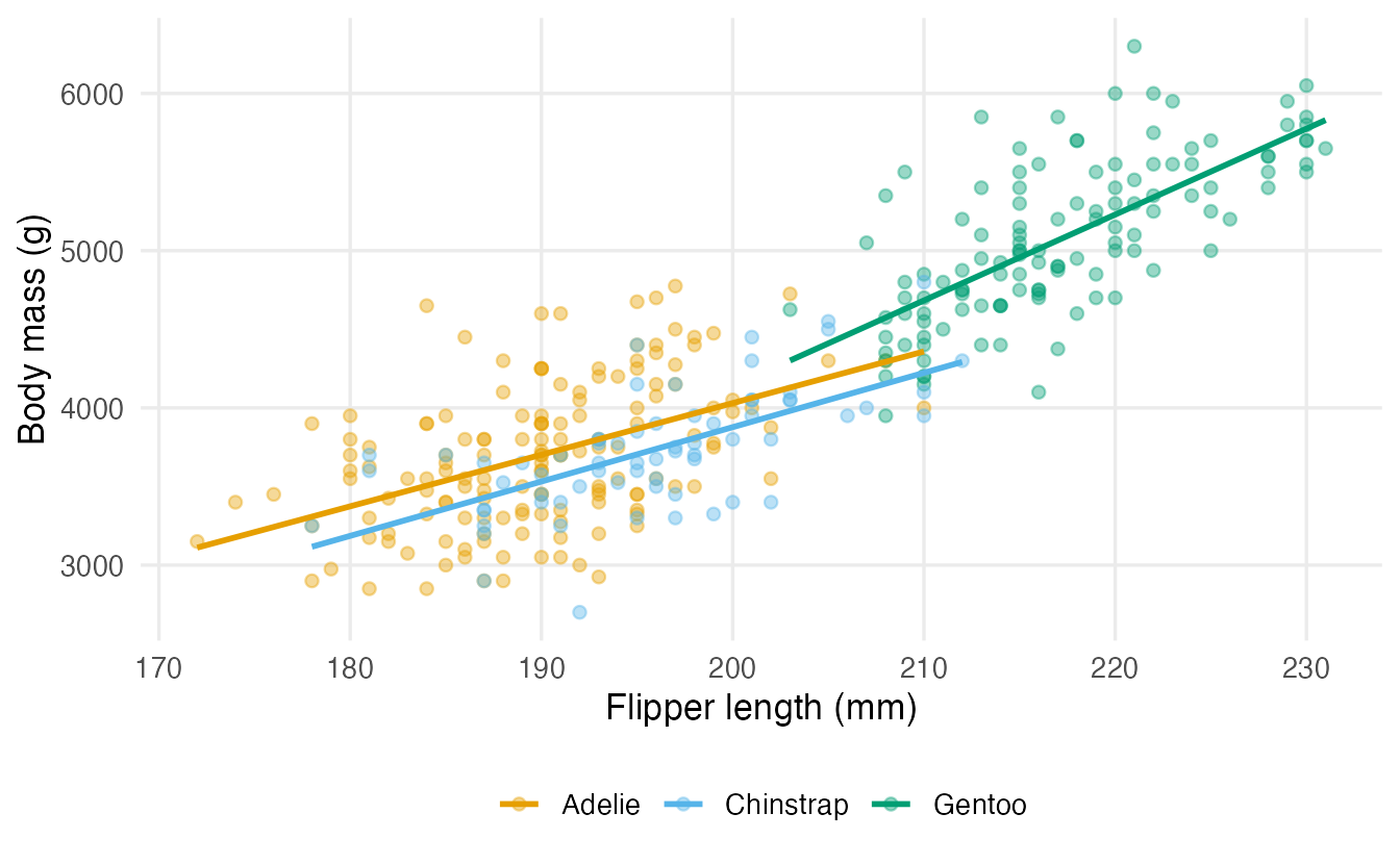
Is the extra flexibility needed? The additive model is nested in the interaction model (it is the special case where both interaction coefficients are 0), so an F-test compares them:
anova(m_add, m_int)#> Analysis of Variance Table
#>
#> Model 1: body_mass ~ flipper_len + species
#> Model 2: body_mass ~ flipper_len * species
#> Res.Df RSS Df Sum of Sq F Pr(>F)
#> 1 338 47666988
#> 2 336 46147424 2 1519564 5.53 0.0043 **
#> ---
#> Signif. codes: 0 '***' 0.001 '**' 0.01 '*' 0.05 '.' 0.1 ' ' 1The p-value (0.0043) suggests that the slopes do differ — mainly because the Gentoo line is steeper. Note that the Chinstrap interaction on its own is far from significant: the overall F-test is the right way to judge “does the interaction matter?”.
NoteGoing deeper: numeric × numeric interactions
With two numeric predictors, y ~ x1 * x2 gives \(\hat y = b_0 + b_1 x_1 + b_2 x_2 + b_3 x_1 x_2\), so the slope of \(x_1\) is \(b_1 + b_3 x_2\): it changes continuously with \(x_2\). Here \(b_1\) is the slope of \(x_1\) when \(x_2 = 0\), which is why centring both variables (subtracting their means) is almost always a good idea before interpreting main effects.
5. Multicollinearity and the VIF
When predictors are strongly correlated with each other, the model struggles to separate their effects: the coefficients become unstable and their standard errors inflated. Consider four correlated car characteristics:
m_four <- lm(mpg ~ disp + hp + wt + drat, data = mtcars)
cor(mtcars[, c("disp", "hp", "wt", "drat")]) |> round(2)
#> disp hp wt drat
#> disp 1.00 0.79 0.89 -0.71
#> hp 0.79 1.00 0.66 -0.45
#> wt 0.89 0.66 1.00 -0.71
#> drat -0.71 -0.45 -0.71 1.00The variance inflation factor of predictor \(j\) is \(\text{VIF}_j = 1/(1 - R_j^2)\), where \(R_j^2\) is the R² from regressing predictor \(j\) on all the other predictors. It says how many times larger the variance of \(\hat\beta_j\) is than it would be with uncorrelated predictors.
car::vif(m_four)#> disp hp wt drat
#> 8.209 2.894 5.097 2.280Let us check one by hand:
r2_disp <- summary(lm(disp ~ hp + wt + drat, data = mtcars))$r.squared
1 / (1 - r2_disp)
#> [1] 8.209Engine displacement is largely predictable from the other three (R² = 0.88), so its standard error is inflated by a factor of about \(\sqrt{8.2} \approx 2.9\). Common rules of thumb flag VIF above 5 or 10.
What to do about it depends on the goal:
- Prediction: collinearity does not hurt predictions within the range of the data; you may leave it alone, or use penalized regression.
- Explanation: you cannot separate effects that the data do not separate. Drop redundant variables, combine them into one index, or accept wide CIs and say so.
For models with factors, car::vif() reports a generalized VIF (GVIF) per term, and GVIF^(1/(2*Df)) is the version comparable to the square root of an ordinary VIF.
6. Influential points: leverage and Cook’s distance
Some observations pull the fitted model more than others.
- Leverage (\(h_{ii}\), from
hatvalues()) measures how unusual an observation’s predictor values are. High-leverage points can move the line a lot. - Cook’s distance combines leverage with the size of the residual: it measures how much all the fitted values would change if the observation were removed.
cd <- cooks.distance(m_wt_hp)
lev <- hatvalues(m_wt_hp)

tibble::tibble(car = names(cd), cooks_d = cd, leverage = lev) |>
  arrange(desc(cooks_d)) |>
  head(4)
#> # A tibble: 4 × 3
#> car cooks_d leverage
#> <chr> <dbl> <dbl>
#> 1 Chrysler Imperial 0.4236 0.1865
#> 2 Maserati Bora 0.2720 0.3942
#> 3 Toyota Corolla 0.2084 0.09950
#> 4 Fiat 128 0.1574 0.07991A common screening threshold is \(4/n\) (= 0.125 here) for Cook’s distance and \(2p/n\) for leverage (\(p\) = number of coefficients). These are flags, not verdicts.
plot(m_wt_hp, which = 5)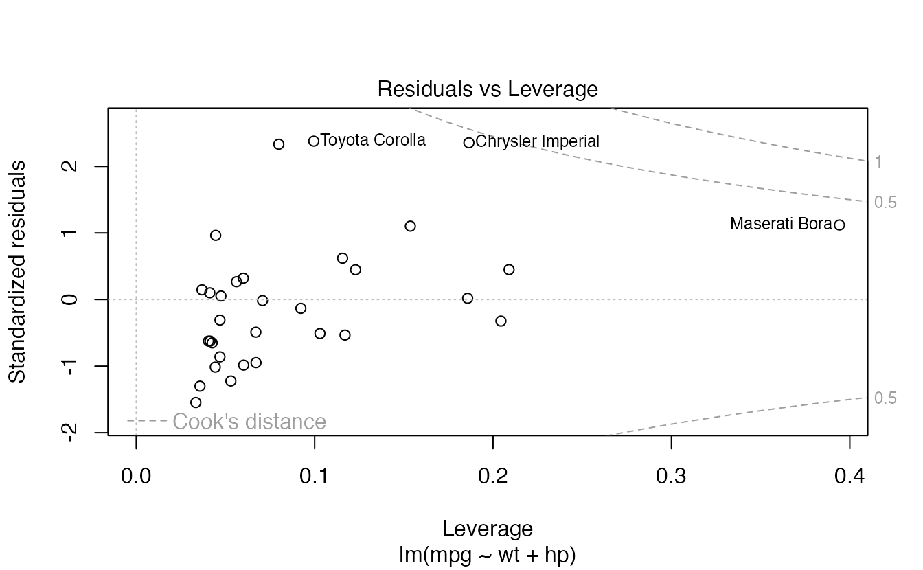
What happens without the most influential car?
worst <- names(which.max(cd))
worst
#> [1] "Chrysler Imperial"update(m_wt_hp, data = mtcars[rownames(mtcars) != worst, ]) |> coef()#> (Intercept) wt hp
#> 38.57947 -4.41966 -0.03055The wt coefficient moves from -3.88 to -4.42. Never delete a point just because it is influential. Check whether it is a data error; if it is genuine, report results with and without it, or use a model that fits it better (here: a curved relationship, see Exercise 5).
7. Heteroscedasticity and robust standard errors
The E of LINE asks for a constant error variance. When the spread of the residuals changes with the fitted values (heteroscedasticity), the coefficients are still unbiased, but the usual standard errors are wrong. A classic example is ozone concentration in New York (airquality):
m_oz <- lm(Ozone ~ Temp + Wind, data = airquality)

augment(m_oz) |>
  ggplot(aes(.fitted, .resid)) +
  geom_hline(yintercept = 0, linetype = 2) +
  geom_point(alpha = 0.6) +
  labs(x = "Fitted ozone (ppb)", y = "Residual")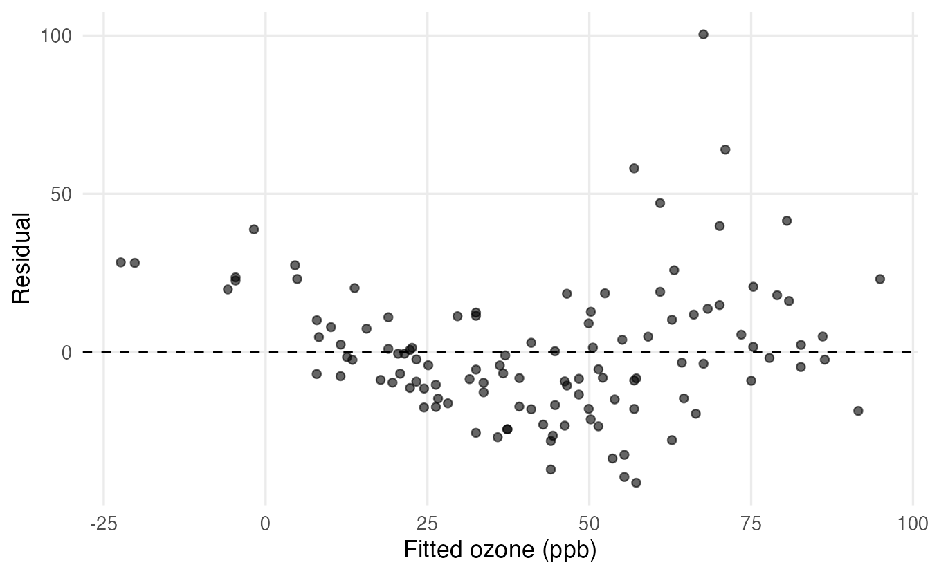
The Breusch–Pagan test asks whether the squared residuals can be predicted from the predictors:
lmtest::bptest(m_oz)#>
#> studentized Breusch-Pagan test
#>
#> data: m_oz
#> BP = 6.1, df = 2, p-value = 0.05A small p-value is evidence of non-constant variance (the plot is usually more informative than the test). Heteroscedasticity-consistent (“robust”, “sandwich”) standard errors remain valid without assuming constant variance:
lmtest::coeftest(m_oz, vcov. = sandwich::vcovHC(m_oz, type = "HC3"))#>
#> t test of coefficients:
#>
#> Estimate Std. Error t value Pr(>|t|)
#> (Intercept) -71.033 22.449 -3.16 0.002 **
#> Temp 1.840 0.203 9.05 4.9e-15 ***
#> Wind -3.055 0.907 -3.37 0.001 **
#> ---
#> Signif. codes: 0 '***' 0.001 '**' 0.01 '*' 0.05 '.' 0.1 ' ' 1Compare with tidy(m_oz): the estimates are identical, but the robust SE of Wind is noticeably larger than the classical one, so the test is less confident. HC3 is a good default for small and moderate samples. Alternatives: transform the response, or use a model whose variance naturally grows with the mean (a GLM).
NoteGoing deeper: the sandwich
The classical covariance is \(\hat\sigma^2 (X^\top X)^{-1}\), which assumes \(\operatorname{Var}(\varepsilon_i) = \sigma^2\) for all \(i\). The sandwich estimator replaces it with
\[ (X^\top X)^{-1} \Big( \sum_i \omega_i\, x_i x_i^\top \Big) (X^\top X)^{-1}, \qquad \omega_i = \frac{e_i^2}{(1 - h_{ii})^2} \ \text{for HC3}, \]
the “bread–meat–bread” shape that gives it its name. Each observation contributes its own squared residual instead of a common \(\hat\sigma^2\).
8. Partial effect plots: showing what the model says
A table of coefficients is hard to read once there are interactions. A partial effect plot shows the model’s predictions as one predictor varies, with the others held at fixed values. We do this with predict() on a grid.
We add sex to the interaction model and plot predicted body mass against flipper length, by species, for female penguins:
m_full <- lm(body_mass ~ flipper_len * species + sex, data = penguins)grid <- penguins |>
filter(!is.na(flipper_len)) |>
group_by(species) |>
reframe(flipper_len = seq(min(flipper_len), max(flipper_len),
length.out = 50)) |>
mutate(sex = factor("female", levels = levels(penguins$sex)))
pred <- predict(m_full, newdata = grid, interval = "confidence")
grid <- bind_cols(grid, as.data.frame(pred))
ggplot(grid, aes(flipper_len, fit, colour = species, fill = species)) +
geom_ribbon(aes(ymin = lwr, ymax = upr), alpha = 0.2, colour = NA) +
geom_line(linewidth = 1) +
labs(x = "Flipper length (mm)", y = "Predicted body mass (g)",
colour = NULL, fill = NULL)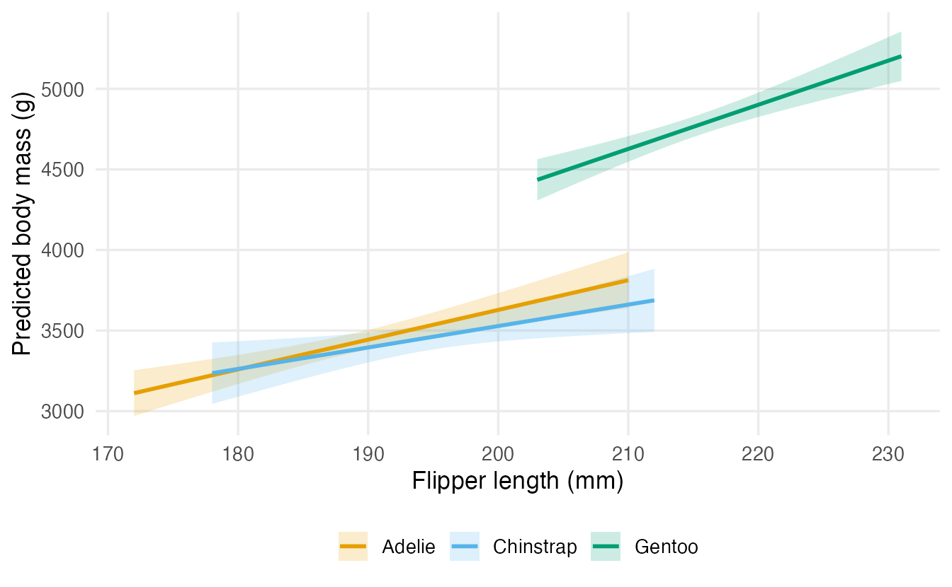
Restricting each line to its species’ observed range avoids extrapolation. Packages such as marginaleffects (plot_predictions()) and ggeffects automate this, but the logic is always the same: build a grid, predict, plot.
Notice that once sex is in the model the species slopes are more similar (anova(lm(body_mass ~ flipper_len + species + sex, data = penguins), m_full) gives p ≈ 0.08). Interactions — like any coefficient — depend on what else is in the model.
9. Reporting a model
A good report states the model, the sample, the key estimates with CIs and units, and how assumptions were checked. For the additive penguin model with sex:
m_report <- lm(body_mass ~ flipper_len + species + sex, data = penguins)
tidy(m_report, conf.int = TRUE) |>
  select(term, estimate, conf.low, conf.high, p.value)
#> # A tibble: 5 × 5
#> term estimate conf.low conf.high p.value
#> <chr> <dbl> <dbl> <dbl> <dbl>
#> 1 (Intercept) -365.8 -1412. 680.8 4.922e- 1
#> 2 flipper_len 20.02 14.43 25.62 1.155e-11
#> 3 speciesChinstrap -87.63 -178.8 3.541 5.953e- 2
#> 4 speciesGentoo 836.3 668.7 1004. 4.112e-20
#> 5 sexmale 530.4 456.0 604.8 2.414e-35glance(m_report) |> select(r.squared, sigma, nobs)#> # A tibble: 1 × 3
#> r.squared sigma nobs
#> <dbl> <dbl> <int>
#> 1 0.8669 295.6 333We modelled body mass (g) as a linear function of flipper length, species and sex (n = 333 penguins with complete data). Holding species and sex constant, each additional millimetre of flipper length was associated with 20 g more body mass (95% CI 14.4 to 25.6). Males were on average 530 g heavier than females of the same species and flipper length (95% CI 456 to 605). The model explained 87% of the variance in body mass; residual plots showed no marked departures from linearity or constant variance.
WarningCommon pitfalls
- Interpreting a main effect in the presence of an interaction as “the” effect. With
x * group, the coefficient ofxis the slope in the reference group only. - Judging a factor by its individual dummies. Whether
speciesmatters is a question for an F-test comparing models, not for one dummy’s p-value — which depends on the arbitrary reference level. - “Controlling for” as magic. Adjustment only removes the confounding of variables you included, measured well. It does not turn observational data into an experiment.
- Deleting influential points to “clean” the data. Investigate them; report sensitivity analyses.
- Including a variable twice. Two versions of the same information (e.g. a factor and its numeric code, or a variable and its sum with others) cause perfect collinearity and
NAcoefficients. - Reading p-values after looking at many models. Choosing predictors based on the data makes the reported p-values too optimistic (see Model selection).
10. Check your understanding
11. Exercises
★ Exercise 1 — reproduce. Fit mpg ~ wt + factor(am) on mtcars (am: 0 = automatic, 1 = manual). Interpret the coefficient of factor(am)1. Then make “manual” the reference level and refit.
TipSolution
cars2 <- mtcars |>
  mutate(am = factor(am, levels = c(0, 1), labels = c("auto", "manual")))
lm(mpg ~ wt + am, data = cars2) |> tidy(conf.int = TRUE)

cars2 |>
  mutate(am = fct_relevel(am, "manual")) |>
  lm(mpg ~ wt + am, data = _) |>
  coef()
Holding weight constant, manual cars have essentially the same mpg as automatics (difference about −0.02, CI from about −3 to 3). The large raw difference in mpg between transmissions is explained by manual cars being lighter. Relevelling only flips the sign of the coefficient.
★★ Exercise 2 — interpret an interaction. From m_int, compute by hand the predicted body mass of a Gentoo with 220 mm flippers and of an Adelie with 190 mm flippers. Check with predict().
TipSolution
b <- coef(m_int)
gentoo_220 <- b["(Intercept)"] + b["speciesGentoo"] +
  (b["flipper_len"] + b["flipper_len:speciesGentoo"]) * 220
adelie_190 <- b["(Intercept)"] + b["flipper_len"] * 190
c(gentoo_220, adelie_190)

predict(m_int, data.frame(flipper_len = c(220, 190),
                          species = c("Gentoo", "Adelie")))
About 5230 g for the Gentoo and about 3700 g for the Adelie. For a Gentoo you add both the Gentoo intercept shift and the Gentoo slope shift.
★★ Exercise 3 — debug. A student writes
penguins2 <- penguins |>
  mutate(is_adelie = species == "Adelie",
         is_chinstrap = species == "Chinstrap",
         is_gentoo = species == "Gentoo")
lm(body_mass ~ is_adelie + is_chinstrap + is_gentoo, data = penguins2)
and gets NA for one coefficient. Explain why and give two ways to fix it.
TipSolution
The three indicators always sum to 1, which equals the intercept column: the design matrix is singular (Section 3, Going deeper). R drops the last one and reports NA. Fixes: (1) leave the coding to R with lm(body_mass ~ species, data = penguins); (2) drop one indicator (it becomes the reference); or (3) drop the intercept with - 1 so that each coefficient is a group mean.
★★ Exercise 4 — collinearity in action. Fit mpg ~ disp, then mpg ~ disp + wt. What happens to the coefficient and the standard error of disp? Compute the VIF of disp in the second model by hand.
TipSolution
tidy(lm(mpg ~ disp, data = mtcars))
tidy(lm(mpg ~ disp + wt, data = mtcars))
1 / (1 - summary(lm(disp ~ wt, data = mtcars))$r.squared)
Alone, disp has a clearly negative slope (about −0.041, SE about 0.005). Together with wt (correlation about 0.89) its slope shrinks to about −0.018, its SE roughly doubles, and it is no longer clearly different from zero. The VIF is about 4.7 (= 1/(1 − 0.89²)). The data cannot tell displacement and weight apart well.
★★★ Exercise 5 — mini-analysis. For mpg ~ wt + hp, (a) draw the four diagnostic plots; (b) add a quadratic term for weight (I(wt^2)) and test whether it improves the fit with anova(); (c) does the most influential car (by Cook’s distance) remain as influential?
TipSolution
par(mfrow = c(2, 2)); plot(m_wt_hp); par(mfrow = c(1, 1))

m_quad <- lm(mpg ~ wt + I(wt^2) + hp, data = mtcars)
anova(m_wt_hp, m_quad)

sort(cooks.distance(m_wt_hp), decreasing = TRUE)[1:3]
sort(cooks.distance(m_quad), decreasing = TRUE)[1:3]
The residuals-vs-fitted plot is U-shaped, a sign of curvature. The quadratic term improves the fit clearly (F-test p ≈ 0.004). The Chrysler Imperial, a very heavy car whose mpg the straight-line model underestimates, has the largest Cook’s distance (about 0.42) in the linear model; in the quadratic model its Cook’s distance drops to about 0.28 because the curve follows it better, and the Maserati Bora (an extreme hp value) becomes the most influential car (about 0.31). Influence is a property of a point and a model.
Summary
| Idea / function | What it does |
|---|---|
lm(y ~ x1 + x2) |
coefficients adjusted for the other predictors |
model.matrix() |
the numeric design matrix (dummies included) |
relevel(), fct_relevel() |
change the reference level of a factor |
y ~ x * group |
interaction: a different slope of x per group |
anova(m_small, m_big) |
F-test for nested models |
car::vif() |
variance inflation factors |
hatvalues(), cooks.distance(), plot(m, which = 5) |
leverage and influence |
lmtest::bptest() |
Breusch–Pagan test of constant variance |
lmtest::coeftest(m, vcov. = sandwich::vcovHC(m)) |
robust standard errors |
predict() on a grid |
partial effect plots |
- Each coefficient in a multiple regression is an association holding the other predictors constant.
- Factors become \(k-1\) dummies; coefficients are differences from the reference level.
- With an interaction, the slope of one predictor depends on the other; visualise it.
- Diagnose collinearity, influence and non-constant variance — and decide what to do based on whether your goal is explanation or prediction.