Penalized regression: ridge, lasso and elastic net

Trading a little bias for a lot of stability — and letting the data choose how much

Why least squares becomes unstable with many or correlated predictors, how ridge, lasso and elastic net shrink coefficients, how to choose the penalty with cross-validation (lambda.min versus lambda.1se), how the lasso selects variables when p > n, and how to tune the same model with tidymodels.

Level 4 · Models & learning ⏱ ~120 min Prerequisites: Multiple regression, Model selection

Learning objectives

By the end of this lesson you will be able to:

explain why least squares becomes unstable with many or correlated predictors, and how a penalty trades bias for variance;
describe ridge, lasso and elastic net and the role of the two tuning parameters $\lambda$ and $\alpha$;
prepare a design matrix correctly and fit penalized models with glmnet, reading coefficient paths and cross-validation curves;
choose $\lambda$ with cv.glmnet() and explain why lambda.1se gives a simpler, more stable model than lambda.min;
compare penalized models with OLS by repeated cross-validation, and tune an elastic net with tidymodels.

library(glmnet)
library(tidymodels)   # rsample, recipes, parsnip, workflows, tune,
                      # yardstick, dials + dplyr, ggplot2, tidyr, tibble

1. Why penalize?

In Model selection we saw that adding predictors always improves the fit to the data at hand, but can make predictions for new data worse, and that choosing predictors with step() is unstable. Let us look at the problem from another angle.

mtcars has 32 cars and 10 candidate predictors of fuel consumption (mpg). We treat cyl, vs and am as categorical:

cars <- mtcars |>
  mutate(cyl = factor(cyl),
         vs = factor(vs),
         am = factor(am, labels = c("auto", "manual")))

m_ols <- lm(mpg ~ ., data = cars)
summary(m_ols)$r.squared

#> [1] 0.8816

summary(m_ols)$coefficients |> round(3)

#>             Estimate Std. Error t value Pr(>|t|)
#> (Intercept)   17.820     16.306   1.093    0.287
#> cyl6          -1.660      2.262  -0.734    0.472
#> cyl8           1.637      4.316   0.379    0.708
#> disp           0.014      0.017   0.799    0.433
#> hp            -0.046      0.027  -1.701    0.104
#> drat           0.026      1.676   0.016    0.988
#> wt            -3.806      1.847  -2.061    0.053
#> qsec           0.647      0.722   0.896    0.381
#> vs1            1.747      2.273   0.769    0.451
#> ammanual       2.617      2.005   1.306    0.207
#> gear           0.764      1.457   0.525    0.606
#> carb           0.509      0.942   0.540    0.595

The model explains 88% of the variance in mpg, yet not a single coefficient is significant at the 5% level. The reason is that the predictors are strongly correlated:

cor(mtcars[, c("cyl", "disp", "hp", "wt")]) |> round(2)

#>       cyl disp   hp   wt
#> cyl  1.00 0.90 0.83 0.78
#> disp 0.90 1.00 0.79 0.89
#> hp   0.83 0.79 1.00 0.66
#> wt   0.78 0.89 0.66 1.00

Big engines (disp), many cylinders, high horsepower and heavy cars go together. With so much overlap, the data cannot tell which of them “really” matters, so the individual coefficients are very uncertain. We can see that uncertainty by refitting the model on bootstrap samples (see The bootstrap):

set.seed(1)
boot_coef <- t(replicate(500, {
  rows <- sample(nrow(cars), replace = TRUE)
  coef(lm(mpg ~ ., data = cars[rows, ]))[c("wt", "disp", "hp")]
}))
colMeans(boot_coef > 0)   # share of bootstrap fits with a positive sign

#>    wt  disp    hp 
#> 0.068 0.798 0.230

The coefficient of engine displacement is positive in 80% of the bootstrap fits and negative in the rest; even horsepower changes sign in 23% of them. Least squares is unbiased but has high variance: small changes in the data produce large changes in the estimates, and in the predictions that depend on them.

Penalized regression accepts a small amount of bias — it pulls (“shrinks”) the coefficients towards zero — in exchange for a large reduction in variance. When predictors are many or correlated, this trade usually improves predictions on new data.

2. The bias–variance trade-off, by simulation

To see the trade in action, we simulate many datasets with two highly correlated predictors (correlation 0.95) and true coefficients $\beta_1 = \beta_2 = 1$. For each dataset we estimate $\beta_1$ by least squares and by ridge regression, which adds a penalty $\lambda$ on the size of the coefficients. Ridge has a closed-form solution that takes a few lines of code (details in the “Going deeper” box of Section 3):

ridge_coef <- function(X, y, lambda) {
  Xc <- scale(X, scale = FALSE)          # centre the predictors
  yc <- y - mean(y)
  n <- nrow(X)
  drop(solve(crossprod(Xc) / n + lambda * diag(ncol(X)),
             crossprod(Xc, yc) / n))
}

set.seed(2026)
sims <- replicate(2000, {
  x1 <- rnorm(30)
  x2 <- 0.95 * x1 + sqrt(1 - 0.95^2) * rnorm(30)   # cor(x1, x2) = 0.95
  y <- 1 * x1 + 1 * x2 + rnorm(30, sd = 2)
  X <- cbind(x1, x2)
  c(OLS = ridge_coef(X, y, 0)[1], ridge = ridge_coef(X, y, 0.5)[1])
})
est <- tibble(method = rep(c("OLS", "ridge"), times = ncol(sims)),
              beta1 = as.vector(sims))
est |>
  summarise(mean = mean(beta1), sd = sd(beta1),
            mse = mean((beta1 - 1)^2), .by = method)

#> # A tibble: 2 × 4
#>   method   mean     sd     mse
#>   <chr>   <dbl>  <dbl>   <dbl>
#> 1 OLS    1.025  1.235  1.524  
#> 2 ridge  0.7867 0.1800 0.07791

ggplot(est, aes(beta1, fill = method)) +
  geom_histogram(binwidth = 0.1, alpha = 0.7, position = "identity") +
  geom_vline(xintercept = 1, linetype = 2) +
  coord_cartesian(xlim = c(-3, 5)) +
  labs(x = expression(hat(beta)[1]), y = "Number of datasets", fill = NULL)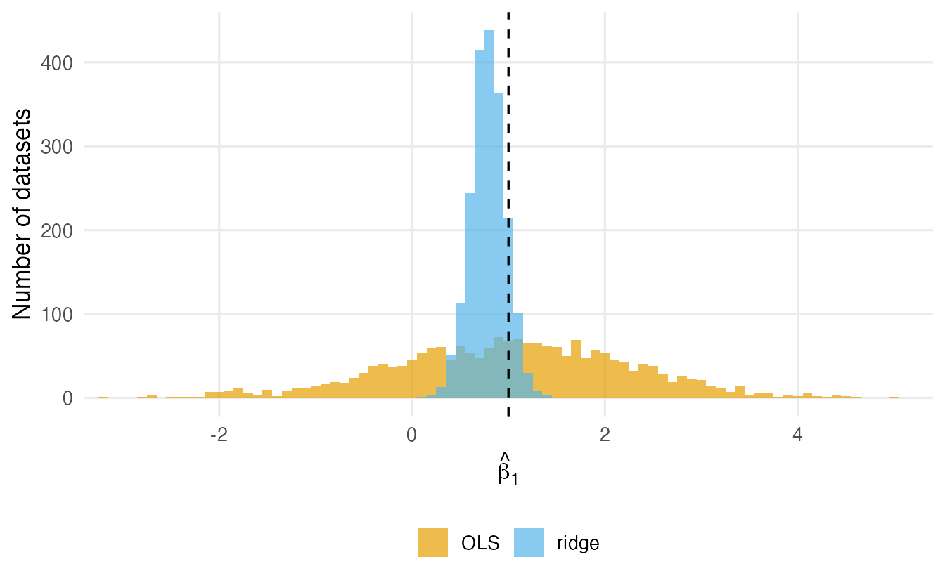

Figure 1: Estimates of a coefficient whose true value is 1 (dashed line) in 2000 simulated datasets. OLS is centred on the truth but very spread out; ridge is slightly biased towards zero but far more precise.

How to read this output

OLS is unbiased (mean 1.02, close to 1) but its estimates have a standard deviation of 1.23: in many datasets it gets even the sign wrong.
Ridge is biased (mean 0.79), but its standard deviation is only 0.18.
The mean squared error (MSE = bias² + variance) is what matters for accuracy: 1.52 for OLS versus 0.08 for ridge. A little bias bought a large gain.

Too much penalty, however, shrinks everything towards zero and the bias dominates (Exercise 6). The amount of penalty, $\lambda$, is a tuning parameter that we will choose by cross-validation.

3. Ridge, lasso and elastic net

All three methods minimise the usual residual sum of squares plus a penalty on the size of the coefficients. The glmnet package, which we use throughout, solves

\[ \min_{\beta_0,\,\beta}\; \underbrace{\frac{1}{2n}\sum_{i=1}^n \big(y_i - \beta_0 - x_i^\top\beta\big)^2}_{\text{fit}} \;+\; \underbrace{\lambda\left[\frac{1-\alpha}{2}\,\lVert\beta\rVert_2^2 + \alpha\,\lVert\beta\rVert_1\right]}_{\text{penalty}}, \]

where $\lVert\beta\rVert_2^2 = \sum_j \beta_j^2$ (sum of squares) and $\lVert\beta\rVert_1 = \sum_j |\beta_j|$ (sum of absolute values). The intercept $\beta_0$ is not penalised.

Method	$\alpha$	Penalty	Typical behaviour
Ridge	0	$\frac{\lambda}{2}\sum_j \beta_j^2$	shrinks all coefficients smoothly; none becomes exactly 0; shares weight among correlated predictors
Lasso	1	$\lambda \sum_j \lvert\beta_j\rvert$	shrinks and sets some coefficients exactly to 0: variable selection
Elastic net	between 0 and 1	a mix of both	selects variables, but keeps groups of correlated predictors together more than the lasso

The two tuning parameters:

$\lambda \ge 0$ sets the strength of the penalty. $\lambda = 0$ gives ordinary least squares; as $\lambda$ grows, coefficients shrink towards 0.
$\alpha \in [0, 1]$ sets the type of penalty (ridge ↔︎ lasso).

Lasso stands for least absolute shrinkage and selection operator.

Standardise the predictors

The penalty treats all coefficients alike, but the size of a coefficient depends on the units of its predictor: the coefficient of weight in tonnes is 1000 times that of weight in kilograms. Without standardisation, the penalty would depend on arbitrary unit choices. glmnet() therefore standardises the predictors internally (standardize = TRUE, the default) and reports the coefficients back on the original scale. In tidymodels we standardise explicitly with step_normalize() in a recipe (Section 10).

Going deeper: the geometry of ridge and lasso

The penalized problem is equivalent to minimising the RSS subject to a budget on the coefficients: $\sum_j \beta_j^2 \le s$ (ridge) or $\sum_j |\beta_j| \le s$ (lasso), where a smaller budget $s$ corresponds to a larger $\lambda$. With two coefficients, the ridge budget is a disc and the lasso budget a diamond:

rss_grid <- tidyr::expand_grid(b1 = seq(-1.5, 3, length.out = 200),
                               b2 = seq(-1.5, 3, length.out = 200)) |>
  mutate(rss = (b1 - 2)^2 + 1.2 * (b1 - 2) * (b2 - 1.2) + (b2 - 1.2)^2)
angle <- seq(0, 2 * pi, length.out = 200)
circle <- tibble(b1 = cos(angle), b2 = sin(angle))
diamond <- tibble(b1 = c(1, 0, -1, 0, 1), b2 = c(0, 1, 0, -1, 0))

ggplot(rss_grid, aes(b1, b2)) +
  geom_contour(aes(z = rss), bins = 12, colour = "grey60") +
  geom_path(data = circle, colour = "#0072B2", linewidth = 1) +
  geom_path(data = diamond, colour = "#D55E00", linewidth = 1) +
  annotate("point", x = 2, y = 1.2, size = 2) +
  annotate("text", x = 2.15, y = 1.35, label = "OLS") +
  geom_hline(yintercept = 0) +
  geom_vline(xintercept = 0) +
  coord_equal() +
  labs(x = expression(beta[1]), y = expression(beta[2]))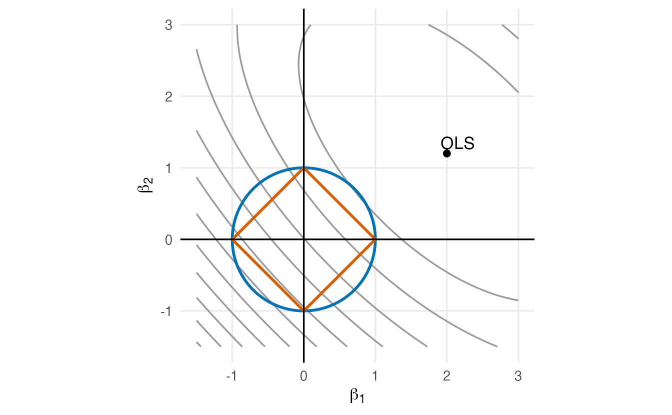

Figure 2: Contours of the residual sum of squares (ellipses, centred on the OLS estimate) and the ridge (circle) and lasso (diamond) constraint regions. The penalized solution is where the smallest ellipse touches the region. The diamond has corners on the axes, so the lasso solution often lands on one, where a coefficient is exactly zero.

The disc has no corners, so the ridge solution almost never has a coordinate exactly equal to 0; it simply moves towards the origin. The diamond’s corners lie on the axes; the first contact with an ellipse frequently happens at a corner, which sets one coefficient to exactly zero. In many dimensions the $\ell_1$ ball has many corners and edges, which is why the lasso produces sparse solutions.

Two more facts:

Ridge has the closed form $\hat\beta_\lambda = (X^\top X/n + \lambda I)^{-1}X^\top y/n$ for centred data (the function ridge_coef() above). Adding $\lambda I$ makes the matrix invertible even when predictors are collinear or $p > n$.
Lasso has no closed form; glmnet uses coordinate descent, updating one coefficient at a time with a “soft-thresholding” step that sets small coefficients to 0. It computes the whole path of solutions for a decreasing sequence of $\lambda$ values very quickly, re-using each solution as the starting point for the next.

4. Preparing the data for glmnet

glmnet() does not take a formula; it needs a numeric matrix x of predictors and a vector y. model.matrix() converts a data frame with factors into such a matrix, creating dummy (indicator) variables for each factor:

X <- model.matrix(mpg ~ ., data = cars)[, -1]   # drop the intercept column
y <- cars$mpg
dim(X)

#> [1] 32 11

colnames(X)

#>  [1] "cyl6"     "cyl8"     "disp"     "hp"       "drat"     "wt"      
#>  [7] "qsec"     "vs1"      "ammanual" "gear"     "carb"

Each factor with $k$ levels becomes $k - 1$ dummy columns: cyl gives cyl6 and cyl8, with 4 cylinders as the reference level. We drop the column of ones ([, -1]) because glmnet fits its own (unpenalised) intercept.

A classic mistake: one dummy too many

A common recipe is model.matrix(mpg ~ . - 1, data = cars). Removing the intercept inside the formula makes R code the first factor with all its levels (cyl4, cyl6, cyl8). If that matrix is later used in a model with an intercept, the three dummies add up to the intercept column — perfect collinearity — and lm() returns NA for one coefficient:

X_bad <- model.matrix(mpg ~ . - 1, data = cars)
coef(lm(y ~ X_bad))[c("X_badcyl4", "X_badcyl6", "X_badcyl8")]

#> X_badcyl4 X_badcyl6 X_badcyl8 
#>    -1.637    -3.298        NA

Use model.matrix(y ~ ., data)[, -1] (one reference level per factor). The penalty would hide the problem in glmnet, but the coefficients of the three cyl dummies would no longer have a clear meaning.

5. Ridge regression with glmnet

glmnet() fits the model for a whole sequence of 100 values of $\lambda$ at once. alpha = 0 gives ridge.

fit_ridge <- glmnet(X, y, alpha = 0)
plot(fit_ridge, xvar = "lambda", label = TRUE)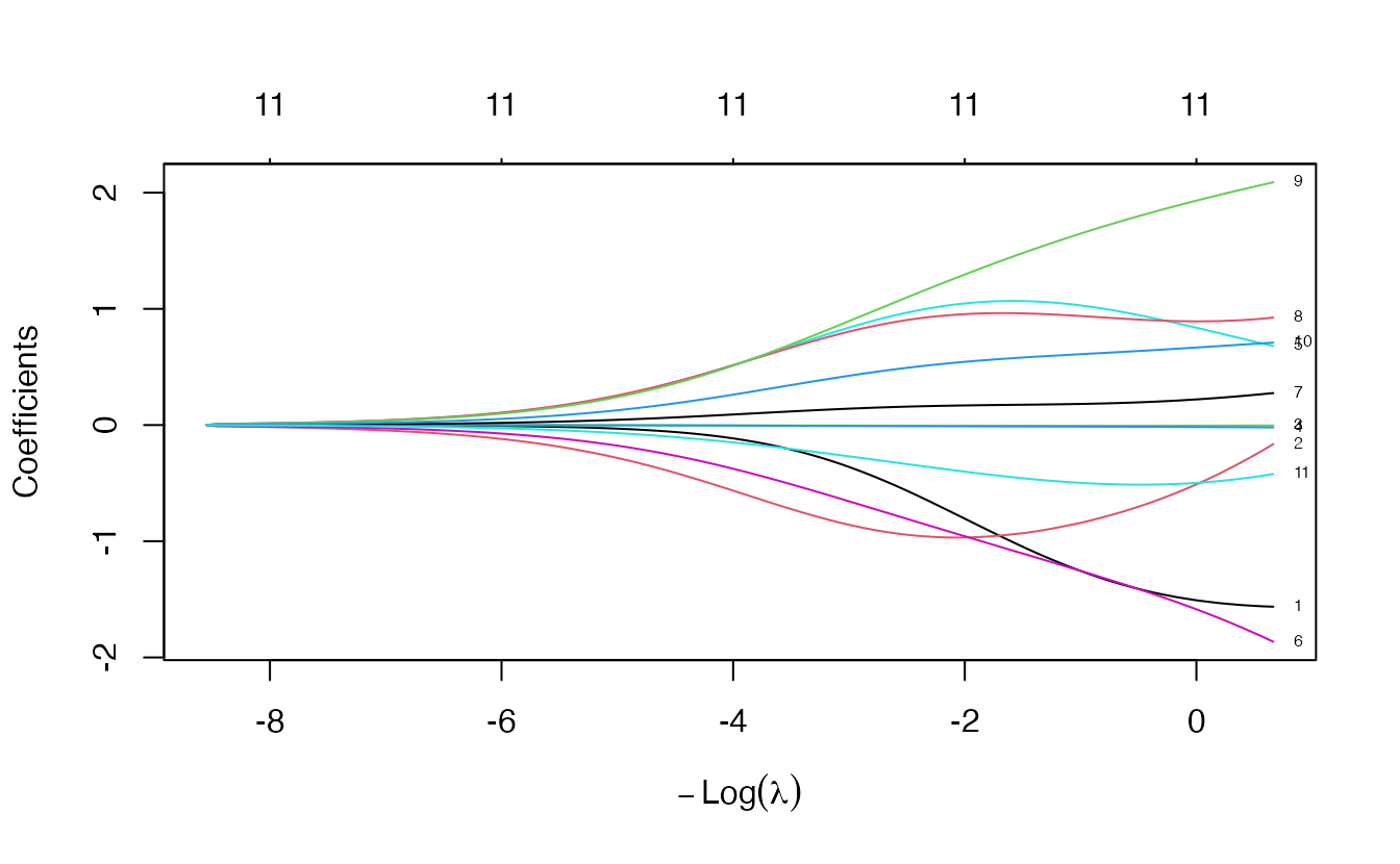

Figure 3: Ridge coefficient paths for the mtcars model. Each line is one coefficient. On the right (large lambda) all coefficients are squeezed towards zero; moving left, the penalty weakens and they approach their OLS values. The numbers on top are the number of non-zero coefficients — always all of them for ridge.

How to read a coefficient path

The x axis is $\log(\lambda)$, increasing to the right. The strongest penalty is on the right, where all coefficients are close to 0; the weakest is on the left, close to OLS.
The y axis shows each coefficient (on the original scale of its predictor); the number at the left end of each line is its column in X (1 = cyl6, 2 = cyl8, and so on).
With ridge no line reaches 0 exactly before the far right; correlated predictors move together.

Which $\lambda$ should we use? The one that predicts new data best — estimated by cross-validation.

6. Choosing $\lambda$ by cross-validation

cv.glmnet() runs $k$-fold cross-validation (10 folds by default) over the whole $\lambda$ sequence and records, for each $\lambda$, the mean CV error and its standard error.

set.seed(123)
cv_ridge <- cv.glmnet(X, y, alpha = 0)
plot(cv_ridge)
c(lambda_min = cv_ridge$lambda.min, lambda_1se = cv_ridge$lambda.1se)

#> lambda_min lambda_1se 
#>      2.503      9.206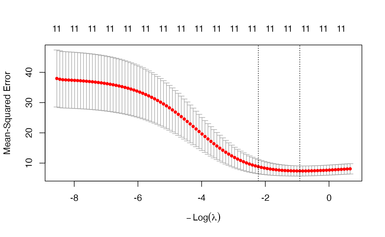

Figure 4: Cross-validated mean squared error of ridge regression as a function of log(lambda), with ±1 standard error bars. The two dotted lines mark lambda.min (left) and lambda.1se (right).

Two values of $\lambda$ are reported:

lambda.min: the $\lambda$ with the lowest mean CV error.
lambda.1se: the largest $\lambda$ whose CV error is within one standard error of the minimum.

lambda.1se applies the one-standard-error rule from Model selection: differences in CV error smaller than their standard error are mostly noise, so among the models that are statistically indistinguishable from the best we choose the most regularised one. It has larger $\lambda$, therefore smaller coefficients and — for the lasso — fewer non-zero coefficients. It is the more parsimonious and more stable choice; lambda.min tends to keep more noise and changes more from one CV run to the next. lambda.min can be preferable when pure predictive accuracy matters more than simplicity and the sample is large.

cbind(min = coef(cv_ridge, s = "lambda.min")[, 1],
      `1se` = coef(cv_ridge, s = "lambda.1se")[, 1],
      ols = coef(m_ols)) |>
  round(3)

#>                min    1se    ols
#> (Intercept) 19.383 17.905 17.820
#> cyl6        -1.285 -0.698 -1.660
#> cyl8        -0.822 -0.965  1.637
#> disp        -0.006 -0.006  0.014
#> hp          -0.014 -0.010 -0.046
#> drat         1.019  1.019  0.026
#> wt          -1.280 -0.891 -3.806
#> qsec         0.183  0.165  0.647
#> vs1          0.933  0.938  1.747
#> ammanual     1.674  1.210  2.617
#> gear         0.614  0.523  0.764
#> carb        -0.502 -0.373  0.509

Overall the coefficients at lambda.1se are pulled further towards zero than at lambda.min, and both sets are more moderate than OLS. Look at cyl8: OLS estimates 1.64 — eight-cylinder cars more economical than four-cylinder ones of the same weight and power, an artefact of collinearity — while ridge at lambda.1se gives -0.97.

We can mark the chosen $\lambda$ on the coefficient path. The path is drawn against $\log(\lambda)$, so the vertical line must be at log(lambda):

plot(fit_ridge, xvar = "lambda")
abline(v = log(cv_ridge$lambda.min), lty = 2)
abline(v = log(cv_ridge$lambda.1se), lty = 3)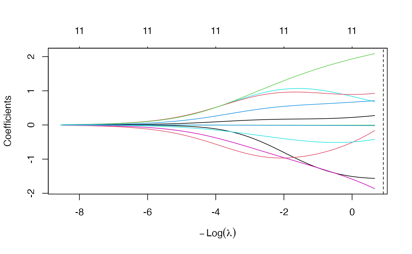

Figure 5: Ridge coefficient paths with lambda.min (dashed) and lambda.1se (dotted).

7. The lasso: shrinkage and selection

alpha = 1 gives the lasso:

fit_lasso <- glmnet(X, y, alpha = 1)
plot(fit_lasso, xvar = "lambda", label = TRUE)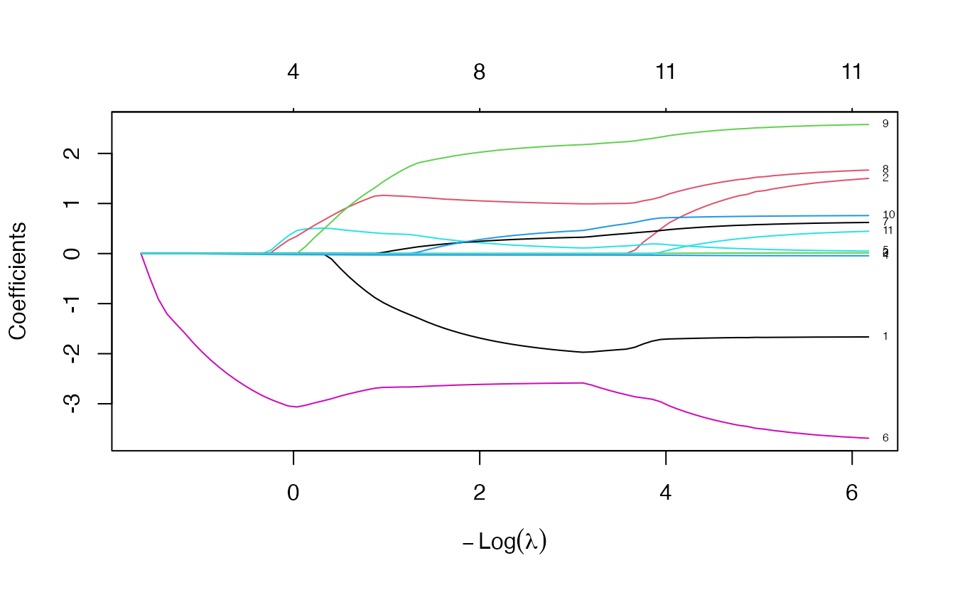

Figure 6: Lasso coefficient paths. Moving from right (strong penalty) to left, predictors enter the model one at a time; the numbers on top count the non-zero coefficients.

set.seed(123)
cv_lasso <- cv.glmnet(X, y, alpha = 1)
plot(cv_lasso)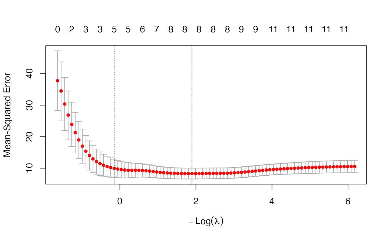

Figure 7: Cross-validated MSE of the lasso. The numbers on top are the number of non-zero coefficients at each lambda.

b_lasso <- cbind(min = coef(cv_lasso, s = "lambda.min")[, 1],
                 `1se` = coef(cv_lasso, s = "lambda.1se")[, 1])
round(b_lasso, 3)

#>                min    1se
#> (Intercept) 25.905 32.006
#> cyl6        -1.642  0.000
#> cyl8         0.000  0.000
#> disp         0.000 -0.001
#> hp          -0.029 -0.020
#> drat         0.233  0.217
#> wt          -2.619 -2.982
#> qsec         0.232  0.000
#> vs1          1.062  0.145
#> ammanual     1.998  0.000
#> gear         0.250  0.000
#> carb         0.000  0.000

colSums(b_lasso[-1, ] != 0)    # non-zero coefficients (excluding intercept)

#> min 1se 
#>   8   5

How to read this output

At lambda.min the lasso keeps 8 predictors; at lambda.1se only 5: disp, hp, drat, wt, vs1.
A coefficient of exactly 0 (printed as 0) means the predictor has been dropped.
The surviving coefficients are shrunk: smaller in absolute value than they would be in an OLS fit with only those predictors.
With strongly correlated predictors, which one the lasso keeps can be somewhat arbitrary: weight and displacement carry much the same information. Do not read the selection as “the other variables do not matter”.

Because cross-validation splits the data at random, lambda.1se and the selected set can change with the seed. Try a few seeds (Exercise 1): this is a reminder that selection from 32 observations is fragile.

8. Elastic net and an honest comparison with OLS

Choosing $\alpha$

The elastic net has two tuning parameters. A simple approach is to run cv.glmnet() for a few values of $\alpha$ using the same folds (foldid), so that the comparison is not distorted by different random splits:

set.seed(2026)
foldid <- sample(rep(1:10, length.out = nrow(X)))
alphas <- c(0, 0.25, 0.5, 0.75, 1)
cv_by_alpha <- lapply(alphas, \(a) cv.glmnet(X, y, alpha = a,
                                             foldid = foldid))

tibble(
  alpha = alphas,
  rmse_min = sapply(cv_by_alpha, \(cv) sqrt(min(cv$cvm))),
  rmse_1se = sapply(cv_by_alpha,
                    \(cv) sqrt(cv$cvm[cv$lambda == cv$lambda.1se])),
  nonzero_1se = sapply(cv_by_alpha,
                       \(cv) cv$nzero[cv$lambda == cv$lambda.1se])
)

#> # A tibble: 5 × 4
#>   alpha rmse_min rmse_1se nonzero_1se
#>   <dbl>    <dbl>    <dbl>       <int>
#> 1  0       2.618    2.893          11
#> 2  0.25    2.712    2.978           8
#> 3  0.5     2.722    2.955           7
#> 4  0.75    2.710    2.939           7
#> 5  1       2.706    2.966           5

cvm is the mean CV squared error, so we take its square root to get an RMSE in mpg. With 32 cars, the differences between values of $\alpha$ are small compared with their uncertainty; what changes clearly is the number of predictors kept.

Does penalization beat OLS here?

The old way to answer this — one train/test split with 8 test cars — gives an answer that depends mostly on which 8 cars were drawn (Model selection, Section 6). Instead we use repeated 5-fold cross-validation. Because cv.glmnet() itself uses cross-validation to choose $\lambda$, it must run inside each training fold (nested CV): the held-out fold must play no part in choosing $\lambda$.

rmse_vec <- function(y, y_hat) sqrt(mean((y - y_hat)^2))

set.seed(2026)
cv_compare <- replicate(10, {
  folds <- sample(rep(1:5, length.out = nrow(X)))
  sapply(1:5, \(i) {
    train <- folds != i
    ols <- lm(mpg ~ ., data = cars[train, ])
    ridge <- cv.glmnet(X[train, ], y[train], alpha = 0, nfolds = 5)
    lasso <- cv.glmnet(X[train, ], y[train], alpha = 1, nfolds = 5)
    c(ols   = rmse_vec(y[!train], predict(ols, cars[!train, ])),
      ridge = rmse_vec(y[!train], predict(ridge, newx = X[!train, ],
                                          s = "lambda.1se")),
      lasso = rmse_vec(y[!train], predict(lasso, newx = X[!train, ],
                                          s = "lambda.1se")))
  }) |>
    rowMeans()
})
cv_rmse <- rowMeans(cv_compare)
round(cv_rmse, 2)

#>   ols ridge lasso 
#>  3.64  2.97  3.21

apply(cv_compare, 1, sd) |> round(2)    # variability across repeats

#>   ols ridge lasso 
#>  0.55  0.11  0.19

How to read this output

Each number is the RMSE (in mpg) for cars not used to fit the model or to choose $\lambda$, averaged over 5 folds × 10 repetitions.
OLS with all 11 coefficients: 3.64; ridge: 2.97; lasso: 3.21 mpg.
The second line shows how much each estimate moves between repetitions — a reminder that differences of a few tenths of a mpg are within the noise for a dataset this small.

The predictors’ standardisation is recomputed by glmnet() within each training fold, and model.matrix() only applies a fixed coding, so nothing leaks from the held-out fold. The real strength of penalization shows when there are many predictors relative to the number of observations — the next section.

9. When $p > n$: lasso as a variable selector

With more predictors than observations, least squares has no unique solution. We simulate 50 observations of 200 predictors, of which only the first 5 truly affect $y$:

set.seed(1)
n <- 50
p <- 200
X_sim <- matrix(rnorm(n * p), nrow = n,
                dimnames = list(NULL, paste0("x", 1:p)))
beta_true <- c(3, -2.5, 2, -1.5, 1, rep(0, p - 5))
y_sim <- drop(X_sim %*% beta_true + rnorm(n))

sum(is.na(coef(lm(y_sim ~ X_sim))))   # coefficients OLS cannot estimate

#> [1] 151

OLS can estimate at most 50 coefficients; 151 are returned as NA, and the 50 it does estimate fit the data perfectly (zero residuals) — useless for prediction. The lasso has no such problem:

set.seed(2)
cv_sim <- cv.glmnet(X_sim, y_sim, alpha = 1)

selected <- function(cv, s) {
  b <- coef(cv, s = s)[-1, 1]
  names(b)[b != 0]
}
sel_min <- selected(cv_sim, "lambda.min")
sel_1se <- selected(cv_sim, "lambda.1se")
true_vars <- paste0("x", 1:5)

tibble(rule = c("lambda.min", "lambda.1se"),
       selected = c(length(sel_min), length(sel_1se)),
       true_found = c(sum(true_vars %in% sel_min),
                      sum(true_vars %in% sel_1se)),
       false_positives = c(sum(!sel_min %in% true_vars),
                           sum(!sel_1se %in% true_vars)))

#> # A tibble: 2 × 4
#>   rule       selected true_found false_positives
#>   <chr>         <int>      <int>           <int>
#> 1 lambda.min       24          5              19
#> 2 lambda.1se       13          5               8

tibble(j = 1:p,
       estimate = coef(cv_sim, s = "lambda.1se")[-1, 1],
       truth = beta_true) |>
  ggplot(aes(j, estimate)) +
  geom_hline(yintercept = 0, colour = "grey60") +
  geom_point(aes(colour = j <= 5)) +
  geom_point(aes(y = truth), shape = 4, size = 2.5) +
  scale_colour_manual(values = c("grey40", "#D55E00"),
                      labels = c("noise", "true signal")) +
  labs(x = "Predictor index", y = "Coefficient", colour = NULL)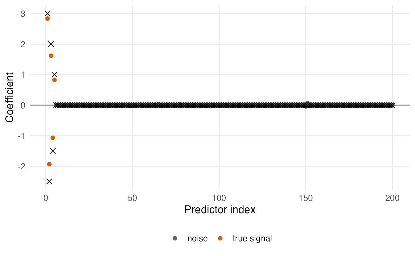

Figure 8: Lasso estimates at lambda.1se for the 200 simulated predictors (points) and true coefficients (crosses). Almost all noise predictors are set exactly to zero; the true ones are found but shrunk towards zero.

How to read this output

At lambda.1se the lasso kept 13 of 200 predictors, including 5 of the 5 true ones and 8 noise variables.
At lambda.min it kept 24: the true signals plus many more noise variables. The smaller penalty buys a slightly lower CV error at the price of a much less parsimonious model.
The estimates of the true coefficients are biased towards zero (the crosses lie farther from 0 than the points). This is the price of the penalty. If clean coefficient estimates are needed, a common two-step approach is to refit OLS on the selected variables — but then the usual p-values are no longer valid (see the box below).

Penalized regression is a prediction tool

glmnet reports no standard errors or p-values, and for good reason: the coefficients are deliberately biased, and the selection of variables was made with the same data. Running lm() on the variables selected by the lasso and reading its p-values has the same problem as stepwise selection (Model selection, Section 4). Valid post-selection inference requires special methods (for example the selectiveInference package) and is beyond this course. Use penalized models when the goal is prediction, or as an exploratory screen.

10. The same with tidymodels

In the machine-learning lessons that follow, models are built with tidymodels (The machine-learning workflow). The glmnet model is linear_reg() with two tuning parameters: penalty (= $\lambda$) and mixture (= $\alpha$).

Recipe — the preprocessing, estimated on the training data inside each resample:

cars_rec <- recipe(mpg ~ ., data = cars) |>
  step_dummy(all_nominal_predictors()) |>       # k - 1 dummies per factor
  step_normalize(all_numeric_predictors())      # mean 0, SD 1

step_dummy() creates $k - 1$ indicator columns per factor (the same coding as model.matrix(...)[, -1]), and step_normalize() standardises every predictor, including the dummies, so that the penalty treats them on a common scale.

Model and workflow:

enet_spec <- linear_reg(penalty = tune(), mixture = tune()) |>
  set_engine("glmnet")

enet_wf <- workflow() |>
  add_recipe(cars_rec) |>
  add_model(enet_spec)

Resamples and grid. With only 32 cars we use repeated 5-fold CV and skip a separate test set; with a larger dataset you would first set one aside with initial_split() and evaluate the final model on it once with last_fit(). (Stratifying the folds by a numeric outcome needs more observations than we have, so we do not use strata here.)

set.seed(2026)
cars_folds <- vfold_cv(cars, v = 5, repeats = 5)

enet_grid <- tidyr::expand_grid(
  penalty = 10^seq(-3, 1, length.out = 30),
  mixture = c(0, 0.25, 0.5, 0.75, 1)
)

enet_res <- tune_grid(enet_wf, resamples = cars_folds, grid = enet_grid,
                      metrics = metric_set(rmse))

autoplot(enet_res)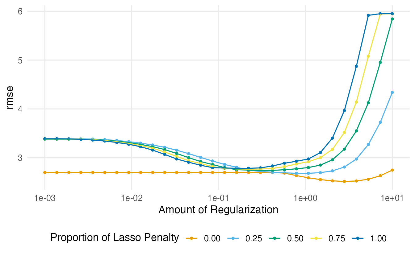

Figure 9: Cross-validated RMSE of the elastic net for each combination of penalty (x axis, log scale) and mixture (colour).

Choosing the parameters:

show_best(enet_res, metric = "rmse", n = 5)

#> # A tibble: 5 × 8
#>   penalty mixture .metric .estimator  mean     n std_err .config          
#>     <dbl>   <dbl> <chr>   <chr>      <dbl> <int>   <dbl> <chr>            
#> 1   2.807       0 rmse    standard   2.515    25  0.1364 pre0_mod126_post0
#> 2   3.857       0 rmse    standard   2.524    25  0.1462 pre0_mod131_post0
#> 3   2.043       0 rmse    standard   2.527    25  0.1281 pre0_mod121_post0
#> 4   1.487       0 rmse    standard   2.553    25  0.1215 pre0_mod116_post0
#> 5   5.298       0 rmse    standard   2.560    25  0.1575 pre0_mod136_post0

best_rmse <- select_best(enet_res, metric = "rmse")
best_1se <- select_by_one_std_err(enet_res, desc(penalty), metric = "rmse")
bind_rows(best = best_rmse, one_se = best_1se, .id = "rule")

#> # A tibble: 2 × 4
#>   rule   penalty mixture .config          
#>   <chr>    <dbl>   <dbl> <chr>            
#> 1 best     2.807       0 pre0_mod126_post0
#> 2 one_se   7.279       0 pre0_mod141_post0

select_best() is the analogue of lambda.min. select_by_one_std_err() implements the one-standard-error rule: among the combinations whose mean RMSE is within one standard error of the best, it returns the simplest, where we define “simplest” by sorting on desc(penalty) — the largest penalty first. This is the analogue of lambda.1se.

Final model — refit on all the data with the chosen parameters:

final_fit <- enet_wf |>
  finalize_workflow(best_1se) |>
  fit(data = cars)

final_fit |>
  extract_fit_parsnip() |>
  tidy() |>
  filter(estimate != 0)

#> # A tibble: 12 × 3
#>    term        estimate penalty
#>    <chr>          <dbl>   <dbl>
#>  1 (Intercept)  20.09     7.279
#>  2 disp         -0.7135   7.279
#>  3 hp           -0.7409   7.279
#>  4 drat          0.5605   7.279
#>  5 wt           -0.9409   7.279
#>  6 qsec          0.3021   7.279
#>  7 gear          0.4024   7.279
#>  8 carb         -0.6507   7.279
#>  9 cyl_X6       -0.3421   7.279
#> 10 cyl_X8       -0.4880   7.279
#> 11 vs_X1         0.4814   7.279
#> 12 am_manual     0.6494   7.279

These coefficients are on the standardised scale (because of step_normalize()): each is the change in mpg for a one-standard-deviation change in the predictor, which makes their sizes directly comparable. The fitted workflow can be used with predict(final_fit, new_data = ...), and the recipe is applied to new data automatically.

Common pitfalls

Calling lambda.min the parsimonious choice. It is the other way round: lambda.1se has the larger penalty, the smaller coefficients and (for the lasso) fewer predictors.
Drawing the chosen $\lambda$ in the wrong place. plot(fit, xvar = "lambda") uses $\log(\lambda)$ on the x axis, so the line is abline(v = log(cv$lambda.1se)), not -log(...).
Including all levels of a factor plus an intercept (model.matrix(y ~ . - 1)). Use model.matrix(y ~ ., data)[, -1] or step_dummy().
Not standardising when you fit penalties outside glmnet (or turning off standardize). The penalty would then depend on the units of measurement.
Judging the model on one tiny test set or choosing $\lambda$ with the data used to evaluate it. Use (repeated, nested) cross-validation.
Reading p-values after lasso selection, or interpreting the lasso’s choice among correlated predictors as evidence that the dropped ones are irrelevant.

11. Check your understanding

Q1. What happens to the lasso coefficients as $\lambda \to 0$? And as $\lambda$ becomes very large?

As $\lambda \to 0$ the penalty vanishes and the coefficients approach the OLS estimates (when OLS exists). As $\lambda$ grows they shrink, one by one they become exactly 0, and for $\lambda$ large enough all of them are 0: the model predicts the mean of $y$ for everyone.

Q2. Why is lambda.1se usually larger than lambda.min?

By definition it is the largest $\lambda$ whose CV error is within one standard error of the minimum. Moving from lambda.min towards larger penalties, the CV error rises slowly at first; lambda.1se is the furthest point before the increase exceeds one standard error.

Q3. You have 10 strongly correlated predictors that all carry similar information. Ridge or lasso?

Ridge (or an elastic net with small $\alpha$) spreads the weight over the correlated group and is stable. The lasso tends to pick one or two of them somewhat arbitrarily, and which ones can change from sample to sample.

Q4. Why must predictors be standardised before applying the penalty?

The penalty is a sum over coefficients, and a coefficient’s size depends on its predictor’s units. Without standardisation, a predictor measured in large units (small coefficient) is barely penalised, and one in small units is heavily penalised — for reasons that have nothing to do with the data.

12. Exercises

★ Exercise 1 — the lasso’s choice is fragile. Run cv.glmnet(X, y, alpha = 1) on the mtcars design matrix with five different seeds. For each run, record lambda.1se and the names of the predictors with non-zero coefficients at lambda.1se. Are the selected sets always the same?

Solution

for (s in 1:5) {
  set.seed(s)
  cv <- cv.glmnet(X, y, alpha = 1)
  b <- coef(cv, s = "lambda.1se")[-1, 1]
  cat("seed", s, ": lambda.1se =", round(cv$lambda.1se, 2), "->",
      names(b)[b != 0], "\n")
}

With only 32 cars, lambda.1se moves noticeably from seed to seed, and so can the number of predictors kept: some predictors (weight, for instance) tend to survive in most runs, others come and go. A more stable choice can be obtained by averaging the CV curves over several runs (or using repeated CV, as in tidymodels), but the lesson is general: variable selection from small samples should be treated with caution.

★★ Exercise 2 — debug. A student plots the lasso path and the chosen penalty with

plot(fit_lasso, xvar = "lambda")
abline(v = -log(cv_lasso$lambda.min), col = "red")

and writes: “I use lambda.min because it gives the most parsimonious model.” Find the two errors.

Solution

The x axis is $\log(\lambda)$, so the line must be at log(cv_lasso$lambda.min). Because $\lambda < 1$ here, $\log(\lambda)$ is negative and $-\log(\lambda)$ is positive: the red line ends up on the wrong side of the plot, at a value of $\lambda$ that was never chosen.
lambda.min is the least regularised of the two standard choices. The parsimonious one is lambda.1se.

plot(fit_lasso, xvar = "lambda")
abline(v = log(cv_lasso$lambda.1se), col = "red")

★★ Exercise 3 — predict the output. Weight wt is in thousands of pounds. Suppose you create X_lb by multiplying the wt column by 1000 (weight in pounds) and refit the lasso. What happens to the coefficient of weight (a) with the default standardize = TRUE, (b) with standardize = FALSE? Check with glmnet(..., lambda = cv_lasso$lambda.1se).

Solution

With standardisation, the fit is the same model: the weight coefficient is simply divided by 1000 and all other coefficients are unchanged. (b) Without it, the coefficient of weight in pounds is tiny, so penalising it costs almost nothing: the lasso keeps weight more easily and the balance with the other predictors changes. The result depends on an arbitrary choice of units — which is why glmnet standardises by default.

X_lb <- X
X_lb[, "wt"] <- X_lb[, "wt"] * 1000
lam <- cv_lasso$lambda.1se
cbind(original = coef(glmnet(X, y, alpha = 1, lambda = lam))[, 1],
      std_true = coef(glmnet(X_lb, y, alpha = 1, lambda = lam))[, 1],
      std_false = coef(glmnet(X_lb, y, alpha = 1, lambda = lam,
                              standardize = FALSE))[, 1]) |>
  round(4)

★★ Exercise 4 — interpret an output. A cv.glmnet() lasso fit reports: lambda.min = 0.08 with 9 non-zero coefficients and CV MSE 7.1; lambda.1se = 0.90 with 3 non-zero coefficients and CV MSE 8.0; the standard error of the CV error at lambda.min is 1.3. Which model would you report and why? What would change your mind?

Solution

The difference in CV MSE (8.0 − 7.1 = 0.9) is smaller than one standard error (1.3): the data cannot really distinguish the two models. The 3-predictor model at lambda.1se is simpler, easier to explain, and its selection is more likely to be reproducible, so it is the natural choice. If small gains in accuracy were valuable (and confirmed on a large test set), or if many repeated CV runs consistently favoured the larger model, lambda.min could be justified.

★★★ Exercise 5 — mini-analysis: how reliable is lasso selection? Repeat the $p > n$ simulation of Section 9 twenty times (new X_sim, y_sim and CV folds each time). For each run, record the number of true predictors found and the number of false positives at lambda.min and at lambda.1se. Summarise the averages.

Solution

set.seed(10)
runs <- replicate(20, {
  Xs <- matrix(rnorm(n * p), nrow = n,
               dimnames = list(NULL, paste0("x", 1:p)))
  ys <- drop(Xs %*% beta_true + rnorm(n))
  cv <- cv.glmnet(Xs, ys, alpha = 1)
  s_min <- selected(cv, "lambda.min")
  s_1se <- selected(cv, "lambda.1se")
  c(true_min = sum(true_vars %in% s_min),
    false_min = sum(!s_min %in% true_vars),
    true_1se = sum(true_vars %in% s_1se),
    false_1se = sum(!s_1se %in% true_vars))
})
rowMeans(runs)

Typically both rules find all or almost all of the 5 true predictors (the weakest, with coefficient 1, is the one most often missed), but lambda.min also lets in many more noise variables than lambda.1se. For variable selection, lambda.1se is clearly the better rule; neither rule is perfect, and the exact counts vary from run to run.

★★ Exercise 6 — bias and variance across $\lambda$. Using ridge_coef() and the simulation of Section 2 (1000 datasets for each value), compute the bias, variance and MSE of $\hat\beta_1$ for $\lambda$ = 0, 0.05, 0.2, 0.5, 2 and 10. Describe the pattern.

Solution

set.seed(2026)
lambdas <- c(0, 0.05, 0.2, 0.5, 2, 10)
bv <- sapply(lambdas, \(l) {
  b1 <- replicate(1000, {
    x1 <- rnorm(30)
    x2 <- 0.95 * x1 + sqrt(1 - 0.95^2) * rnorm(30)
    y <- x1 + x2 + rnorm(30, sd = 2)
    ridge_coef(cbind(x1, x2), y, l)[1]
  })
  c(lambda = l, bias = mean(b1) - 1, variance = var(b1),
    mse = mean((b1 - 1)^2))
})
round(t(bv), 3)

As $\lambda$ grows the variance falls steadily (from about 1.5 at $\lambda = 0$ to almost 0), while the bias grows in magnitude (from about 0 to about −0.84 at $\lambda = 10$). The MSE first drops sharply, reaches its minimum around $\lambda = 0.5$ (about 0.08), then rises again as the bias dominates (about 0.7 at $\lambda = 10$). This U-shape is the bias–variance trade-off; cross-validation is a way to find the bottom of the U without knowing the truth.

Summary

Idea / function	What it does
`model.matrix(y ~ ., data)[, -1]`	numeric design matrix with $k-1$ dummies per factor
`glmnet(X, y, alpha = 0 / 1 / 0.5)`	ridge / lasso / elastic net path over many $\lambda$
`plot(fit, xvar = "lambda")`, `abline(v = log(lambda))`	coefficient paths against $\log\lambda$
`cv.glmnet(X, y, alpha, foldid = )`	CV error over the $\lambda$ path
`lambda.min`, `lambda.1se`	best CV error; most regularised within 1 SE (simpler, more stable)
`coef(cv, s = "lambda.1se")`, `predict(cv, newx, s = )`	coefficients and predictions at a chosen $\lambda$
`linear_reg(penalty = tune(), mixture = tune()) \\|> set_engine("glmnet")`	the same model in tidymodels
`step_dummy()`, `step_normalize()`	dummy coding and standardisation inside a recipe
`tune_grid()`, `select_best()`, `select_by_one_std_err(..., desc(penalty))`	tuning and the one-standard-error rule

Penalization shrinks coefficients, trading a little bias for a large reduction in variance.
Ridge keeps all predictors; the lasso sets some exactly to zero; the elastic net mixes the two.
Standardise predictors so that the penalty does not depend on units (glmnet does it by default).
Choose $\lambda$ by cross-validation; lambda.1se is the parsimonious, stable choice.
Evaluate with repeated, nested CV, and treat penalized models as prediction tools, not sources of p-values.

Penalized regression: ridge, lasso and elastic net

1. Why penalize?

2. The bias–variance trade-off, by simulation

3. Ridge, lasso and elastic net

4. Preparing the data for glmnet

5. Ridge regression with glmnet

6. Choosing \(\lambda\) by cross-validation

7. The lasso: shrinkage and selection

8. Elastic net and an honest comparison with OLS

Choosing \(\alpha\)

Does penalization beat OLS here?

9. When \(p > n\): lasso as a variable selector

10. The same with tidymodels

11. Check your understanding

12. Exercises

Summary