Confidence intervals

Estimate ± margin of error — and what “95% confident” really means

Build confidence intervals for a mean, a proportion and a difference in means, check by simulation what the confidence level promises, and learn to interpret intervals correctly.

Level 3 · Inference ⏱ ~70 min Prerequisites: Sampling distributions, Bootstrap

Learning objectives

By the end of this lesson you will be able to:

build a confidence interval for a mean by hand and with t.test();
build a confidence interval for a proportion and explain why the simple “Wald” interval can fail;
simulate the coverage of an interval and explain what the confidence level promises;
predict how sample size and confidence level change the width of an interval;
interpret a confidence interval correctly and spot the common wrong interpretations.

library(dplyr)
library(ggplot2)

1. Why a single number is not enough

The mean flipper length of the Adelie penguins in our data is about 190 mm. If a different team of researchers caught a different set of Adelie penguins, they would get a slightly different mean. In Sampling distributions we saw how much such estimates vary from sample to sample; in Bootstrap we estimated that variability by resampling.

A point estimate (one number) hides this uncertainty. A confidence interval (CI) reports a range instead:

estimate ± margin of error

The margin of error is “a few standard errors”: it tells the reader how far from the truth our estimate could plausibly be, given the size and noisiness of the sample.

2. A confidence interval for a mean, by hand

The recipe has three ingredients:

the estimate: the sample mean $\bar x$;
the standard error (SE): how much $\bar x$ typically varies between samples, $s / \sqrt{n}$;
a multiplier that sets the confidence level. For 95% and a mean, we use the 97.5% quantile of a t distribution with $n - 1$ degrees of freedom (close to 2 for moderate $n$).

adelie <- penguins |>
  filter(species == "Adelie", !is.na(flipper_len)) |>
  pull(flipper_len)

n      <- length(adelie)
x_bar  <- mean(adelie)
se     <- sd(adelie) / sqrt(n)
t_crit <- qt(0.975, df = n - 1)

c(lower = x_bar - t_crit * se, upper = x_bar + t_crit * se)

#> lower upper 
#> 188.9 191.0

With $n =$ 151 birds the standard error is only 0.53 mm and the multiplier is 1.976, so the margin of error is 1.05 mm.

t.test() does the same calculation (and much more — see t-tests). The interval is stored in $conf.int:

ci_adelie <- t.test(adelie)$conf.int
ci_adelie

#> [1] 188.9 191.0
#> attr(,"conf.level")
#> [1] 0.95

How to read this output

The two numbers are the lower and upper limits: 188.9 to 191 mm.
attr(,"conf.level") reminds you of the confidence level used (0.95 by default; change it with conf.level = 0.90, for example).
In words: “Our best estimate of the mean flipper length of Adelie penguins is 190 mm; values between 188.9 and 191 mm are compatible with the data.”

Going deeper: why the t distribution?

If the data come from a normal population, the standardised mean

\[ T = \frac{\bar X - \mu}{S / \sqrt{n}} \]

follows a t distribution with $n-1$ degrees of freedom. Therefore $P(-t_{0.975} \le T \le t_{0.975}) = 0.95$, and rearranging the inequality for $\mu$ gives the interval

\[ \bar x \pm t_{n-1,\,0.975}\,\frac{s}{\sqrt n}. \]

We use $t$ rather than the normal quantile 1.96 because $s$ is itself an estimate: the extra uncertainty makes the tails heavier. The difference matters only for small samples: qt(0.975, 4) is 2.78, qt(0.975, 29) is 2.05, and qnorm(0.975) is 1.96. Thanks to the Central Limit Theorem the interval also works for non-normal data when $n$ is large enough — see Exercise 3 for a case where “large enough” matters.

3. What “95%” really means: a simulation

Here is the most important idea of the lesson. The “95%” is not a property of one interval. It is a property of the method: if we repeated the whole study many times, building an interval each time, about 95% of those intervals would contain the true value.

We can check this, because in a simulation we choose the truth. Let us invent a population with true mean $\mu = 50$ and standard deviation 10, draw 100 samples of size 20, and build 100 intervals.

set.seed(2026)
mu <- 50

cis <- replicate(100, t.test(rnorm(20, mean = mu, sd = 10))$conf.int)

sims <- tibble(
  id     = 1:100,
  lower  = cis[1, ],
  upper  = cis[2, ],
  covers = lower <= mu & mu <= upper
)
sum(sims$covers)

#> [1] 96

ggplot(sims, aes(y = id, colour = covers)) +
  geom_segment(aes(x = lower, xend = upper, yend = id), linewidth = 0.7) +
  geom_vline(xintercept = mu, linetype = "dashed") +
  scale_colour_manual(values = c(`TRUE` = "grey60", `FALSE` = "#D55E00"),
                      labels = c(`TRUE` = "contains 50",
                                 `FALSE` = "misses 50")) +
  labs(x = "95% confidence interval", y = "Sample number", colour = NULL)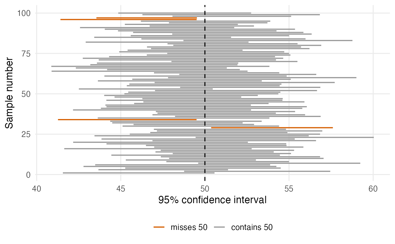

Figure 1: 100 confidence intervals from 100 samples of the same population. The dashed line is the true mean. Intervals that miss it are highlighted.

In this run, 96 of the 100 intervals contain the true mean and 4 miss it. Run it again with another seed and you will get a slightly different count, but close to 95. Notice two things in the figure:

the intervals move (their centres are different sample means) and have different widths (each uses its own $s$);
the true mean does not move. It is fixed; it is the intervals that are random.

With more repetitions the proportion settles very close to 0.95:

set.seed(1)
covers <- replicate(5000, {
  ci <- t.test(rnorm(20, mean = mu, sd = 10))$conf.int
  ci[1] <= mu & mu <= ci[2]
})
mean(covers)

#> [1] 0.9468

The correct interpretation

“We used a method that captures the true mean in 95% of repeated samples. Applied to our sample, it gives the interval [a, b].”

Once you have computed your interval, the true mean is either inside it or not — you just do not know which. The 95% describes how often the procedure works, not the probability for this one interval.

4. What makes an interval wide or narrow?

The margin of error is multiplier × $s / \sqrt n$. So:

larger $n$ → smaller SE → narrower interval. Because of the square root, to halve the width you need about four times as many observations;
higher confidence level → larger multiplier → wider interval. More confidence costs precision;
more variable data (larger $s$) → wider interval.

widths <- expand.grid(n = 5:100, level = c(0.90, 0.95, 0.99)) |>
  mutate(width = 2 * qt(1 - (1 - level) / 2, df = n - 1) / sqrt(n),
         level = factor(paste0(level * 100, "%")))

ggplot(widths, aes(n, width, colour = level)) +
  geom_line(linewidth = 1) +
  labs(x = "Sample size n", y = "Interval width (in SD units)",
       colour = "Confidence level")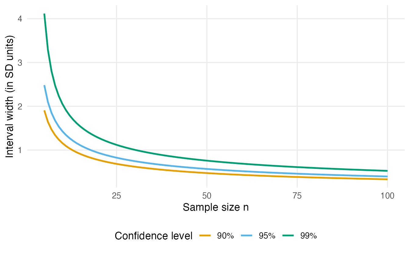

Figure 2: Expected width of a t-based interval (population SD = 1) as a function of sample size, for three confidence levels.

The same trade-off with real data:

sapply(c(0.90, 0.95, 0.99), \(lev) t.test(adelie, conf.level = lev)$conf.int)

#>       [,1]  [,2]  [,3]
#> [1,] 189.1 188.9 188.6
#> [2,] 190.8 191.0 191.3

Each column is one interval (90%, 95%, 99%): they share the same centre and get wider as the level increases.

5. A confidence interval for a proportion

For a yes/no variable the estimate is the sample proportion $\hat p = x / n$ and its standard error is $\sqrt{\hat p (1 - \hat p) / n}$. The textbook (“Wald”) interval is

\[ \hat p \pm 1.96 \sqrt{\hat p (1 - \hat p) / n}. \]

Let us estimate the proportion of females among the penguins whose sex is recorded:

n_known  <- sum(!is.na(penguins$sex))
x_female <- sum(penguins$sex == "female", na.rm = TRUE)
p_hat    <- x_female / n_known

wald <- p_hat + c(-1, 1) * qnorm(0.975) * sqrt(p_hat * (1 - p_hat) / n_known)
wald

#> [1] 0.4418 0.5492

R offers two better intervals:

prop.test(x_female, n_known)$conf.int    # Wilson score interval

#> [1] 0.4407 0.5504
#> attr(,"conf.level")
#> [1] 0.95

binom.test(x_female, n_known)$conf.int   # Clopper-Pearson "exact" interval

#> [1] 0.4405 0.5505
#> attr(,"conf.level")
#> [1] 0.95

With 333 birds and $\hat p$ close to 0.5, the three intervals are practically identical. The trouble starts with small samples or proportions near 0 or 1. Suppose 2 of 20 patients have a side effect:

p_small <- 2 / 20
p_small + c(-1, 1) * qnorm(0.975) * sqrt(p_small * (1 - p_small) / 20)

#> [1] -0.03148  0.23148

binom.test(2, 20)$conf.int

#> [1] 0.01235 0.31698
#> attr(,"conf.level")
#> [1] 0.95

The Wald interval has a negative lower limit — an impossible proportion. The interval from binom.test() stays inside [0, 1] and is asymmetric, as it should be when $\hat p$ is near the boundary.

The deeper problem is coverage. We can simulate it exactly as before: the true proportion is 0.10 and $n = 20$.

set.seed(3)
x_sim <- rbinom(5000, size = 20, prob = 0.10)

wald_covers <- sapply(x_sim, \(x) {
  p <- x / 20
  abs(p - 0.10) <= qnorm(0.975) * sqrt(p * (1 - p) / 20)
})
exact_covers <- sapply(x_sim, \(x) {
  ci <- binom.test(x, 20)$conf.int
  ci[1] <= 0.10 & 0.10 <= ci[2]
})
c(wald = mean(wald_covers), exact = mean(exact_covers))

#>   wald  exact 
#> 0.8796 0.9884

The “95%” Wald interval actually captures the truth only about 88% of the time, while the exact interval covers at least 95% (it is deliberately conservative). Recommendation: use prop.test() or binom.test() and treat the Wald formula as a teaching device.

Going deeper: Wilson and Clopper–Pearson

Wilson (used by prop.test(), with a continuity correction by default) inverts the score test: it collects all values $p_0$ for which $|\hat p - p_0| / \sqrt{p_0(1-p_0)/n} \le 1.96$. The SE is evaluated at $p_0$, not at $\hat p$, which keeps the interval inside [0, 1] and gives coverage close to 95% even for small $n$.
Clopper–Pearson (used by binom.test()) inverts the exact binomial test. Its coverage is never below the nominal level, so it tends to be a little wide.
The Wald interval fails because when $\hat p$ is near 0 or 1, $\sqrt{\hat p (1-\hat p)/n}$ underestimates the true SE (with $x = 0$ it is exactly 0: an interval of width zero!).

Proportions are tested formally in Proportions and chi-square tests.

6. A confidence interval for a difference in means

Very often the question is a comparison: how much heavier are male Adelie penguins than females? The same logic applies — estimate ± multiplier × SE — with the SE of a difference.

adelie_sex <- penguins |>
  filter(species == "Adelie", !is.na(sex))

ci_diff <- t.test(body_mass ~ sex, data = adelie_sex)$conf.int
ci_diff

#> [1] -776.3 -573.0
#> attr(,"conf.level")
#> [1] 0.95

The interval refers to female − male (R orders the groups alphabetically): females are, on average, between 573 and 776 g lighter. The interval does not contain 0, so “no difference” is not a value compatible with the data. The full story — Welch’s test, paired data, effect sizes — is in t-tests.

7. Right and wrong interpretations

Suppose a study reports a 95% CI for a mean of [12.1, 15.3].

Statement	Correct?
“If we repeated the study many times, about 95% of the intervals computed this way would contain the true mean.”	✅ Yes — this is the definition.
“Values between 12.1 and 15.3 are compatible with the data; values far outside are not.”	✅ Yes — a useful practical reading.
“There is a 95% probability that the true mean is between 12.1 and 15.3.”	❌ No. The true mean is fixed; this particular interval either contains it or not.
“95% of the observations lie between 12.1 and 15.3.”	❌ No. The CI is about the mean, not individual values. Individual values are far more spread out.
“A second sample would give a mean between 12.1 and 15.3 with probability 95%.”	❌ No. The next sample mean has its own variability; this probability is noticeably lower than 95%.
“Two intervals that overlap mean the groups do not differ significantly.”	❌ Not necessarily. Two 95% CIs can overlap a little even when the difference is significant. Build a CI for the difference instead.

Common pitfalls

Reading a CI as a probability statement about the parameter. The 95% is about the long-run behaviour of the method.
Confusing the CI for a mean with the range of the data. With large $n$ the CI becomes very narrow, while the data stay as spread out as ever.
Using the Wald interval for small samples or extreme proportions. It can leave [0, 1] and under-covers. Use binom.test() or prop.test().
Comparing groups by checking whether their separate CIs overlap. Compute the interval of the difference.
Forgetting what the interval cannot fix. A CI accounts for random sampling error only. A biased sample (for example, only the penguins that were easy to catch) gives a precise interval around the wrong value.

8. Check your understanding

Q1. You quadruple the sample size. What happens, roughly, to the width of a 95% CI for a mean?

It is roughly halved, because the standard error is proportional to $1/\sqrt{n}$ and $\sqrt{4} = 2$.

Q2. A colleague computes a 99% CI and a 90% CI from the same data. Which one is wider, and why?

The 99% interval. To capture the true value more often, the method must cast a wider net, so it uses a larger multiplier.

Q3. In the simulation of Section 3, why did some intervals miss the true mean?

Because by chance those samples had a mean far from 50 (or an unusually small standard deviation). A 95% method is expected to miss in about 5% of samples — this is not a mistake in the code.

Q4. In a survey, 0 of 15 people report a rare condition. What does the Wald interval give, and what should you use instead?

The Wald interval is $0 \pm 0$, i.e. [0, 0], which would claim we are certain the proportion is zero. binom.test(0, 15)$conf.int gives a sensible interval from 0 to about 0.22.

9. Exercises

Interactive (run in your browser)

★ Exercise 1 — CI for a mean. Compute the 95% and the 90% confidence intervals for the mean mpg in mtcars. Which one is narrower?

ci95 <- t.test(mtcars$mpg)$conf.int
ci90 <- t.test(mtcars$mpg, conf.level = 0.90)$conf.int
ci95   # about 17.9 to 22.3
ci90   # about 18.3 to 21.9

The 90% interval is narrower: lower confidence buys more precision.

★★ Exercise 2 — Wald versus exact. In a small pilot study 3 of 15 participants dropped out. Compute the Wald 95% interval by hand and compare it with binom.test(). What is wrong with the Wald interval here?

se <- sqrt(p_hat * (1 - p_hat) / n)
wald <- p_hat + c(-1, 1) * qnorm(0.975) * se
wald                         # about -0.002 to 0.40
binom.test(x, n)$conf.int    # about 0.04 to 0.48

The Wald interval dips below zero (an impossible proportion) and is symmetric even though $\hat p = 0.2$ is close to the boundary. The exact interval is asymmetric and stays within [0, 1].

★★★ Exercise 3 — does 95% always mean 95%? Data from an exponential distribution (rate 1, true mean 1) are strongly skewed. Simulate 5,000 samples of size n = 10, build the t-based 95% interval each time and estimate its coverage. Then repeat with n = 50. What do you observe?

covers <- replicate(5000, {
  x  <- rexp(n, rate = 1)
  ci <- t.test(x)$conf.int
  ci[1] <= 1 & 1 <= ci[2]
})
mean(covers)   # about 0.90 with n = 10; about 0.93 with n = 50

With skewed data and a small sample, the “95%” interval covers the truth only about 90% of the time. With larger $n$ the Central Limit Theorem kicks in and coverage moves towards 95%. The confidence level is a promise that holds only if the assumptions hold (or $n$ is large enough). For skewed data, a bootstrap interval (Bootstrap) or a transformation can help.

Practice on your own computer

★★ Exercise 4 — one interval per group. For each penguin species, compute the mean bill length (bill_len) and its 95% CI, and plot the three intervals with geom_pointrange().

Solution

bill_ci <- penguins |>
  filter(!is.na(bill_len)) |>
  summarise(
    mean  = mean(bill_len),
    lower = t.test(bill_len)$conf.int[1],
    upper = t.test(bill_len)$conf.int[2],
    .by = species
  )
bill_ci

ggplot(bill_ci, aes(x = species, y = mean, ymin = lower, ymax = upper)) +
  geom_pointrange() +
  labs(x = NULL, y = "Mean bill length (mm) with 95% CI")

Adelie bills are clearly shorter (interval roughly 38.4 to 39.2 mm); the Chinstrap and Gentoo intervals (roughly 48.0–49.6 and 47.0–48.1 mm) are close to each other. To decide whether those two species differ, build an interval for their difference (Section 6), not by eye.

★★ Exercise 5 — interpret. A news article says: “The average commuting time is 32 minutes (95% CI 30 to 34). So 95% of commuters travel between 30 and 34 minutes.” Explain the error in two sentences and rewrite the second sentence correctly.

Solution

The interval is about the average commuting time, not about individual commuters: individual times vary far more (many people travel 10 or 60 minutes). A correct sentence is: “Average commuting times between 30 and 34 minutes are compatible with the data; the method used captures the true average in 95% of repeated surveys.”

Summary

Idea / function	What it does
estimate ± multiplier × SE	General recipe for a confidence interval
`qt(0.975, df = n - 1)`	t multiplier for a 95% CI for a mean
`t.test(x)$conf.int`	CI for a mean (`conf.level =` to change the level)
`t.test(y ~ g, data = df)$conf.int`	CI for a difference in means
`prop.test(x, n)$conf.int`	Wilson CI for a proportion
`binom.test(x, n)$conf.int`	Exact (Clopper–Pearson) CI for a proportion

The confidence level describes the method: in repeated samples about 95% of intervals contain the truth.
The parameter is fixed; the interval is random.
Width shrinks with $\sqrt n$ and grows with the confidence level and with the variability of the data.
For proportions, avoid the Wald interval with small $n$ or extreme $\hat p$.
A CI covers sampling error only — not bias in how the data were collected.