Multidimensional scaling

From a table of distances back to a map

Learn classical (metric) MDS with cmdscale(), why non-Euclidean distances produce negative eigenvalues, how to judge the fit with GOF and Shepard diagrams, non-metric MDS with isoMDS(), and MDS on non-geographic dissimilarities.

Level 4 · Models & learning ⏱ ~75 min Prerequisites: Principal component analysis, Matrices

Learning objectives

By the end of this lesson you will be able to:

explain what a dissimilarity matrix is and what MDS tries to do with it;
run classical MDS with cmdscale() and read its eigenvalues and goodness of fit;
recognise non-Euclidean dissimilarities from negative eigenvalues;
check a configuration with a Shepard diagram, and run non-metric MDS with MASS::isoMDS();
apply MDS to dissimilarities between objects that are not places (variables, mixed-type observations).

library(dplyr)
library(ggplot2)
library(MASS, include.only = c("isoMDS", "Shepard"))   # avoid masking dplyr::select

1. Why MDS?

Sometimes we do not have variables for our objects, only how different they are from each other: road distances between cities, how often people confuse two sounds, how dissimilar two products are judged to be, the genetic distance between species. Such a table is a dissimilarity matrix: a symmetric table with zeros on the diagonal, where entry \((i, j)\) says how far object \(i\) is from object \(j\).

Multidimensional scaling (MDS) answers: can I place the objects as points on a plane (or in a few dimensions) so that the distances between points reproduce the dissimilarities? If it works, the plot is a map of the objects, and we can look at it to find groups, gradients and outliers.

2. A table of road distances

eurodist contains the road distances (in km) between 21 European cities — not straight-line distances, and not all capitals (Calais, Cherbourg, Gibraltar, Hook of Holland, Lyons, Marseilles, Milan, Munich are included).

class(eurodist)

#> [1] "dist"

as.matrix(eurodist)[1:5, 1:5]

#>           Athens Barcelona Brussels Calais Cherbourg
#> Athens         0      3313     2963   3175      3339
#> Barcelona   3313         0     1318   1326      1294
#> Brussels    2963      1318        0    204       583
#> Calais      3175      1326      204      0       460
#> Cherbourg   3339      1294      583    460         0

It is stored as a dist object: only the lower triangle is kept, because the table is symmetric.

3. Classical MDS with `cmdscale()`

mds_euro <- cmdscale(eurodist, k = 2, eig = TRUE)
names(mds_euro)

#> [1] "points" "eig"    "x"      "ac"     "GOF"

head(round(mds_euro$points), 4)

#>           [,1] [,2]
#> Athens    2290 1799
#> Barcelona -825  547
#> Brussels    59 -367
#> Calais     -83 -430

points are the coordinates of the cities in a two-dimensional configuration. Classical MDS (also called principal coordinates analysis, PCoA) is closely related to PCA: it computes eigenvalues and eigenvectors of a matrix derived from the distances, and keeps the first k dimensions.

Eigenvalues: some are negative!

round(mds_euro$eig / 1e6, 2)          # in millions, for readability

#>  [1] 19.54 11.86  1.53  1.12  0.79  0.58  0.26  0.19  0.15  0.11  0.05  0.00
#> [13] -0.01 -0.05 -0.13 -0.26 -0.33 -0.52 -0.92 -1.01 -2.25

sum(mds_euro$eig < 0)

#> [1] 10

If the distances were Euclidean (straight-line distances between points in some space), all eigenvalues would be \(\ge 0\). Here 10 eigenvalues are negative, the largest in absolute value being -2.25 million. Negative eigenvalues are the signature of non-Euclidean dissimilarities: no configuration of points, in any number of dimensions, reproduces road distances exactly. Roads bend around mountains and seas, and the Earth is not flat.

The negative eigenvalues are small compared with the first two (19.5 and 11.9 million), so a 2-D map is still a good summary.

Goodness of fit

cmdscale() returns two goodness-of-fit (GOF) measures for the k dimensions kept, with eigenvalues \(\lambda_1, \lambda_2, \dots\):

\[ \text{GOF}_1 = \frac{\sum_{i=1}^{k} \lambda_i}{\sum_{i} |\lambda_i|}, \qquad \text{GOF}_2 = \frac{\sum_{i=1}^{k} \lambda_i}{\sum_{i} \max(\lambda_i, 0)} . \]

mds_euro$GOF

#> [1] 0.7538 0.8679

How to read the GOF

GOF₂ = 0.868: the two dimensions account for 87% of the sum of the positive eigenvalues.
GOF₁ = 0.754 is smaller because its denominator also includes the absolute values of the negative eigenvalues — that is, it penalises the non-Euclidean part of the data.
For Euclidean distances the two values coincide. A large gap between them is another sign that the dissimilarities are far from Euclidean.

4. Turning the configuration into a map

cities <- data.frame(city = labels(eurodist),
                     dim1 = mds_euro$points[, 1],
                     dim2 = mds_euro$points[, 2])

ggplot(cities, aes(dim1, dim2, label = city)) +
  geom_point() +
  geom_text(vjust = -0.6, size = 3) +
  coord_equal() +
  labs(x = "Dimension 1 (km)", y = "Dimension 2 (km)")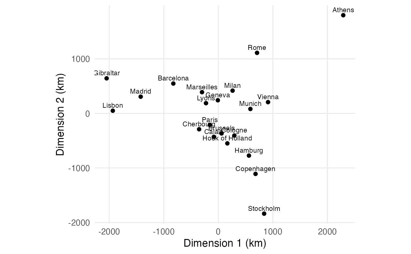

Figure 1: Raw classical MDS configuration of the 21 cities, before any flipping.

Distances alone carry no information about orientation: rotating or mirroring the map does not change any distance. The signs of the MDS axes, like those of PCA components, are arbitrary. To make the map look like Europe we want west on the left and north at the top. Instead of guessing, we let the data decide using three cities we know:

if (cities$dim1[cities$city == "Lisbon"] > cities$dim1[cities$city == "Athens"]) {
  cities$dim1 <- -cities$dim1        # Lisbon must be west of Athens
}
if (cities$dim2[cities$city == "Stockholm"] < cities$dim2[cities$city == "Athens"]) {
  cities$dim2 <- -cities$dim2        # Stockholm must be north of Athens
}

With the configuration R returns here, axis 1 already had west on the left, while axis 2 had to be flipped (north was at the bottom). On another computer the signs may differ — which is exactly why we test instead of hard-coding a flip.

ggplot(cities, aes(dim1, dim2, label = city)) +
  geom_point(colour = "#0072B2") +
  geom_text(vjust = -0.6, size = 3) +
  coord_equal() +
  labs(x = "West – East (km)", y = "South – North (km)")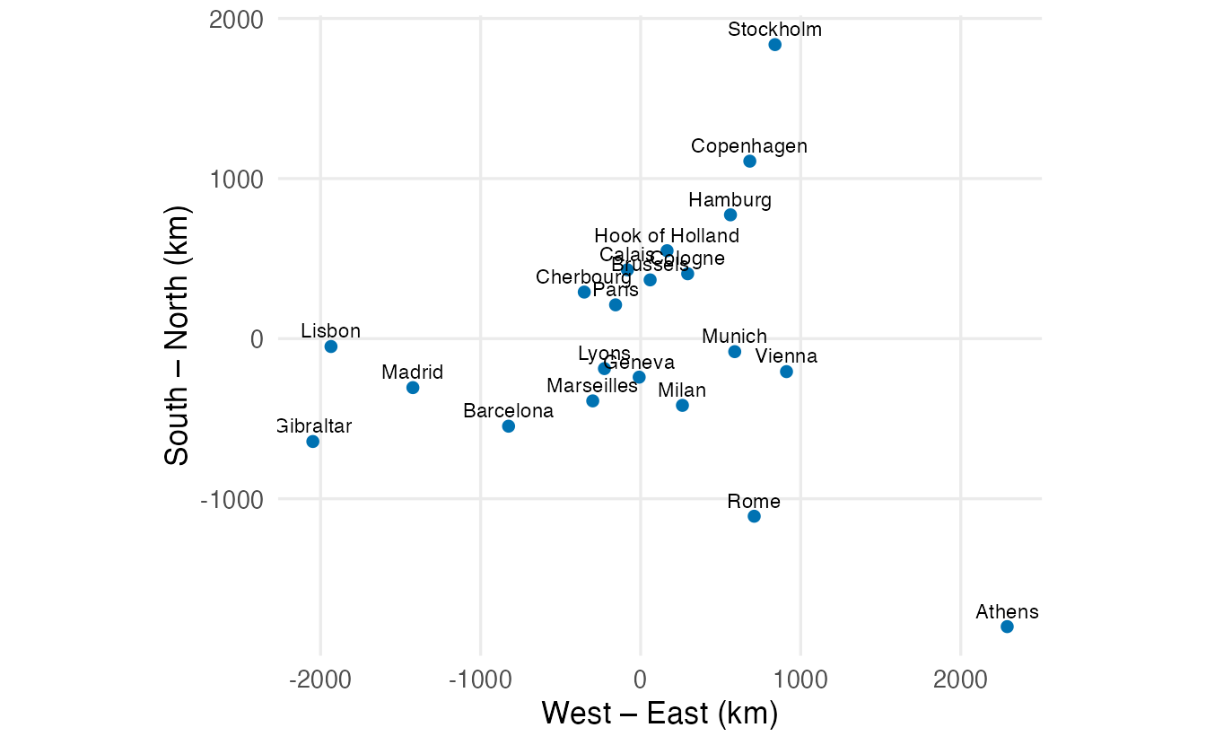

Figure 2: Classical MDS map of 21 European cities from road distances, oriented with west on the left and north at the top.

Reading the map

The Iberian cities (Lisbon, Madrid, Gibraltar, and Barcelona further east) are on the far left.
Stockholm and Copenhagen are at the top (north), with Hamburg below them.
Athens is in the far south-east, and Rome south of Milan.
The North Sea and Channel cities (Calais, Brussels, Hook of Holland, Cherbourg) and Paris form a cluster in the north-west centre; Geneva, Lyons and Marseilles lie between this cluster and the Mediterranean.

The geography is recognisable, but not perfect: the map is built from road distances, not coordinates.

Going deeper: double centring

Let \(D^{(2)}\) be the matrix of squared dissimilarities and \(J = I - \frac1n \mathbf 1 \mathbf 1^\top\) the centring matrix. Classical MDS computes

\[ B = -\tfrac12 \, J D^{(2)} J , \]

the double-centred matrix (rows and columns centred). If the dissimilarities are Euclidean distances between points \(x_1, \dots, x_n\), then \(B\) is exactly the matrix of inner products of the centred points, \(B = XX^\top\), which is positive semi-definite. Writing \(B = V \Lambda V^\top\), the coordinates are \(X_k = V_k \Lambda_k^{1/2}\) — this is what cmdscale() returns. When the dissimilarities are not Euclidean, \(B\) has negative eigenvalues and \(\Lambda^{1/2}\) only exists for the positive ones.

D2 <- as.matrix(eurodist)^2
n  <- nrow(D2)
J  <- diag(n) - matrix(1 / n, n, n)
B  <- -0.5 * J %*% D2 %*% J
e  <- eigen(B, symmetric = TRUE)

X  <- e$vectors[, 1:2] %*% diag(sqrt(e$values[1:2]))
all.equal(abs(X), abs(unname(mds_euro$points)))   # same up to sign

#> [1] TRUE

5. How good is the map? Shepard diagram

A Shepard diagram plots the original dissimilarities against the distances on the map. If the map were perfect, all points would lie on the diagonal.

fitted_d <- dist(mds_euro$points)

shep <- data.frame(road = as.vector(eurodist),
                   map  = as.vector(fitted_d))

ggplot(shep, aes(road, map)) +
  geom_point(alpha = 0.5) +
  geom_abline(slope = 1, intercept = 0, colour = "#D55E00") +
  labs(x = "Road distance (km)", y = "Distance on the MDS map (km)")

cor(shep$road, shep$map)

#> [1] 0.986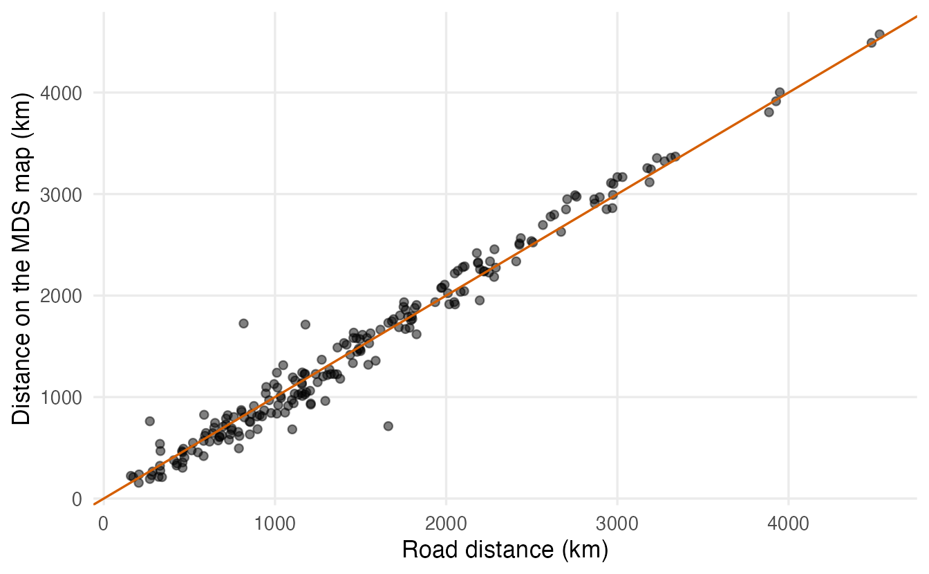

Figure 3: Shepard diagram: road distances versus distances on the 2-D MDS map. Each point is a pair of cities.

The correlation between road and map distances is 0.986. Most pairs are close to the diagonal. Which pairs are worst?

pairs <- t(combn(labels(eurodist), 2))   # same order as the dist object
shep |>
  mutate(from = pairs[, 1], to = pairs[, 2], error = map - road) |>
  arrange(desc(abs(error))) |>
  head(4)

#>   road    map       from              to  error
#> 1 1662  713.3    Cologne          Geneva -948.7
#> 2  817 1724.7     Athens            Rome  907.7
#> 3 1178 1714.2     Lisbon           Lyons  536.2
#> 4  269  761.6 Copenhagen Hook of Holland  492.6

Some entries cannot be reproduced by any flat map. For instance the table gives Athens–Rome as 817 km, which is shorter than the straight-line distance between the two cities (about 1,050 km). A few entries of this old table look inconsistent with geography, and MDS spreads their error over the whole map.

6. Non-metric MDS

Classical MDS tries to reproduce the dissimilarities as numbers. Often we only trust their order: “A is more similar to B than to C”. Rating scales, rankings and many ecological dissimilarities are like this. Non-metric MDS looks for a configuration whose distances are in the same rank order as the dissimilarities, as far as possible.

The mismatch is measured by Kruskal’s stress (0 = perfect). MASS::isoMDS() reports it in percent. Kruskal’s rough guide: below 5% good, 5–10% fair, 10–20% poor, above 20% bad.

iso_euro <- isoMDS(eurodist, k = 2, trace = FALSE)  # starts from cmdscale()
iso_euro$stress

#> [1] 7.506

sh <- Shepard(eurodist, iso_euro$points)
plot(sh, pch = 20, col = "grey50",
     xlab = "Road distance (km)", ylab = "Map distance")
lines(sh$x, sh$yf, type = "S", col = "#D55E00", lwd = 2)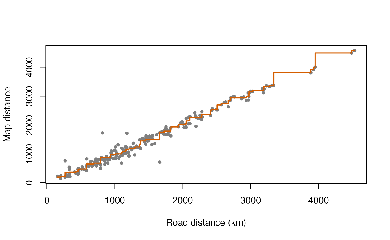

Figure 4: Shepard diagram for non-metric MDS: the step line is the best monotone (order-preserving) fit.

The stress is 7.5%. For road distances, metric and non-metric MDS give very similar maps; non-metric MDS really pays off when only the order of the dissimilarities is meaningful.

7. MDS beyond geography: a map of variables

MDS works with any dissimilarity. Let’s draw a map of the 11 variables of mtcars, using a distance based on their correlation: strongly positively correlated variables should be close, negatively correlated ones far apart.

\[ d_{jk} = \sqrt{2(1 - r_{jk})} \]

This is (up to a constant) the Euclidean distance between the standardised variables, so it ranges from 0 (\(r = 1\)) to 2 (\(r = -1\)).

d_vars  <- as.dist(sqrt(2 * (1 - cor(mtcars))))
mds_var <- cmdscale(d_vars, k = 2, eig = TRUE)

round(mds_var$eig, 3)

#>  [1] 6.608 2.437 0.506 0.264 0.217 0.164 0.135 0.078 0.070 0.022 0.000

mds_var$GOF

#> [1] 0.8614 0.8614

Because this distance is Euclidean, there are no (meaningfully) negative eigenvalues and the two GOF values coincide — a nice contrast with eurodist.

data.frame(variable = rownames(mds_var$points), mds_var$points) |>
  ggplot(aes(X1, X2, label = variable)) +
  geom_point() +
  geom_text(vjust = -0.7) +
  coord_equal() +
  labs(x = "Dimension 1", y = "Dimension 2")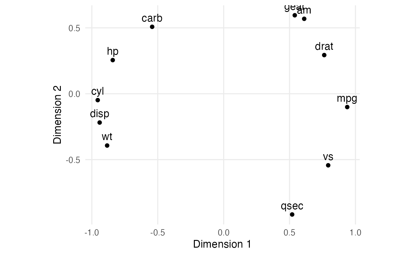

Figure 5: MDS map of the variables of mtcars, from the distance sqrt(2(1 - r)).

mpg lies on the opposite side of the map from cyl, disp and wt (strong negative correlations), and close to drat and vs. The second dimension separates qsec from am, gear and carb. This is the same structure that PCA of mtcars revealed in the PCA lesson — but seen from the variables’ side.

Common pitfalls

Assuming every distance table is Euclidean. Road distances, Gower distances, rating-based dissimilarities usually are not; check the eigenvalues.
Misreading GOF. It is a pair of ratios of eigenvalue sums (with absolute or positive eigenvalues in the denominator), not squared values to be added.
Interpreting the orientation or signs of MDS axes. Distances are unchanged by rotation and reflection; flip axes freely to make the map readable, and decide flips from the data, not by hard-coding them.
Forgetting coord_equal() / asp = 1. Unequal axis scales distort distances on the plot.
Comparing isoMDS() stress with stress values reported as proportions. isoMDS() reports percent.

8. Check your understanding

Q1. Classical MDS on a dissimilarity matrix returns some negative eigenvalues. What does that tell you?

The dissimilarities are not Euclidean: no configuration of points in any dimension reproduces them exactly. If the negative eigenvalues are small relative to the leading positive ones, a low-dimensional map can still be a good approximation.

Q2. Two analysts get mirror-image MDS maps from the same distances. Who is right?

Both. Reflections (and rotations) leave all distances unchanged, so both configurations fit equally well.

Q3. When would you prefer non-metric MDS to classical MDS?

When only the rank order of the dissimilarities is trustworthy (ratings, rankings, many similarity judgements), or when the relation between dissimilarity and distance is expected to be non-linear.

9. Exercises

★ Exercise 1 — MDS of Euclidean distances = PCA. Compute the Euclidean distances between the 150 flowers of iris after standardising the four measurements (dist(scale(iris[, 1:4]))). Run cmdscale(..., k = 2, eig = TRUE) and compare the coordinates with the first two PCA scores of prcomp(iris[, 1:4], scale. = TRUE). Are there negative eigenvalues?

Solution

d_iris <- dist(scale(iris[, 1:4]))
mds_iris <- cmdscale(d_iris, k = 2, eig = TRUE)
pca_iris <- prcomp(iris[, 1:4], scale. = TRUE)
all.equal(abs(unname(mds_iris$points)), abs(unname(pca_iris$x[, 1:2])))
range(mds_iris$eig)      # smallest values are ~0 (rounding), not truly negative

The coordinates coincide up to sign: classical MDS of Euclidean distances is PCA. Apart from numerical rounding (tiny values around ±1e-13), there are no negative eigenvalues.

★ Exercise 2 — predict. You multiply all entries of eurodist by 0.621 to convert kilometres into miles and rerun cmdscale(). What happens to (a) the shape of the map, (b) the eigenvalues, (c) the GOF?

Solution

Same shape, just scaled by 0.621. (b) Eigenvalues are multiplied by 0.621² (they are in squared units). (c) GOF is unchanged — it is a ratio of eigenvalues.

m_miles <- cmdscale(eurodist * 0.621, k = 2, eig = TRUE)
m_miles$eig[1] / mds_euro$eig[1]    # 0.621^2
m_miles$GOF

★★ Exercise 3 — debug. This code is supposed to draw the map with north at the top, but on a colleague’s computer Stockholm ends up at the bottom. Why, and how would you make it robust?

pts <- cmdscale(eurodist)
pts[, 2] <- -pts[, 2]
plot(pts, type = "n", asp = 1); text(pts, labels(eurodist))

Solution

The sign of each MDS axis is arbitrary and can differ between computers or R/BLAS versions; the code flips axis 2 unconditionally. Decide the flip from the data:

pts <- cmdscale(eurodist)
if (pts["Stockholm", 2] < pts["Athens", 2]) pts[, 2] <- -pts[, 2]
if (pts["Lisbon", 1] > pts["Athens", 1]) pts[, 1] <- -pts[, 1]
plot(pts, type = "n", asp = 1); text(pts, labels(eurodist), cex = 0.7)

★★ Exercise 4 — a third dimension. Run classical MDS of eurodist with k = 3. How much do GOF₁ and GOF₂ increase compared with k = 2? Is the third dimension worth keeping?

Solution

cmdscale(eurodist, k = 2, eig = TRUE)$GOF
cmdscale(eurodist, k = 3, eig = TRUE)$GOF

The third eigenvalue is much smaller than the first two (about 1.5 million vs 19.5 and 11.9 million), so GOF increases only modestly (GOF₂ from about 0.87 to about 0.91, GOF₁ from about 0.75 to about 0.79). For a geographic map two dimensions are the natural choice; the extra dimension mostly absorbs distortions of the road network.

★★★ Exercise 5 — mixed data with Gower distance. Penguins are described by numeric measurements and categorical variables (island, sex). The Gower dissimilarity handles both: numeric differences are divided by the variable’s range, categorical variables contribute 0 (same) or 1 (different), and everything is averaged. (a) Compute the Gower dissimilarity with cluster::daisy(..., metric = "gower") on island, sex, bill_len, bill_dep, flipper_len, body_mass (complete cases). (b) Run classical MDS and colour the points by species. (c) Are there negative eigenvalues? (d) What do the two dimensions seem to capture?

Solution

peng <- penguins |>
  select(species, island, sex, bill_len, bill_dep, flipper_len, body_mass) |>
  na.omit()

d_gower <- cluster::daisy(peng |> select(-species), metric = "gower")
mds_g <- cmdscale(d_gower, k = 2, eig = TRUE)
sum(mds_g$eig < 0)
mds_g$GOF

data.frame(mds_g$points, species = peng$species, sex = peng$sex) |>
  ggplot(aes(X1, X2, colour = species, shape = sex)) +
  geom_point(alpha = 0.7) +
  coord_equal()

There are many negative eigenvalues (Gower dissimilarity is not Euclidean) and GOF₁ is clearly smaller than GOF₂. In the map, one dimension separates Gentoo (different island and body shape) from Adelie and Chinstrap, which largely overlap; the other dimension separates females from males — the categorical variable sex creates a 0/1 jump that dominates a whole dimension. That is a property of the Gower distance worth remembering: categorical variables can weigh a lot.

Summary

Idea / function	What it does
`dist()`, `as.dist()`	build a dissimilarity object
`cmdscale(d, k, eig = TRUE)`	classical (metric) MDS: `points`, `eig`, `GOF`
negative `eig`	the dissimilarities are not Euclidean
`GOF`	\(\sum_{i \le k}\lambda_i\) over \(\sum\|\lambda_i\|\) and over \(\sum \max(\lambda_i, 0)\)
Shepard diagram	original vs fitted distances
`MASS::isoMDS()`	non-metric MDS; stress in percent
`cluster::daisy(metric = "gower")`	dissimilarity for mixed numeric/categorical data

MDS turns a table of dissimilarities into a map whose distances approximate them.
Classical MDS of Euclidean distances is PCA; non-Euclidean inputs give negative eigenvalues.
Orientation and signs are arbitrary: flip axes based on the data to make the map readable.
Judge the map with GOF, a Shepard diagram and, for non-metric MDS, stress.

1. Why MDS?

2. A table of road distances

3. Classical MDS with cmdscale()

Eigenvalues: some are negative!

Goodness of fit

4. Turning the configuration into a map

5. How good is the map? Shepard diagram

6. Non-metric MDS

7. MDS beyond geography: a map of variables

8. Check your understanding

9. Exercises

Summary

3. Classical MDS with `cmdscale()`