Factor analysis

Uncover the latent traits behind questionnaire items — and judge whether the model holds

Learn the factor model, how it differs from PCA, how to check factorability, choose the number of factors, use polychoric correlations for Likert items, rotate obliquely, read loadings and fit indices, and assess reliability with alpha and omega.

Level 4 · Models & learning ⏱ ~100 min Prerequisites: Principal component analysis, Correlation

NoteLearning objectives

By the end of this lesson you will be able to:

• explain the factor model \(X = \Lambda F + \varepsilon\) and how it differs from PCA (common vs total variance);
• check whether data are suitable for factor analysis (KMO, Bartlett) and choose the number of factors with parallel analysis and theory;
• fit an exploratory factor analysis with psych::fa() using polychoric correlations and an oblique rotation;
• interpret loadings, communalities, uniquenesses, factor correlations and fit indices;
• compute factor scores and the reliability of a scale (Cronbach’s α, McDonald’s ω), handling reverse-keyed items.

library(dplyr)
library(ggplot2)
library(psych)    # fa(), fa.parallel(), KMO(), alpha(), omega(); needs GPArotation for oblimin

1. Why factor analysis?

Personality questionnaires ask things like “I am the life of the party” or “I get stressed out easily” on a 1–6 scale. Nobody cares about any single item for its own sake. We care about the traits behind them — extraversion, neuroticism — which we cannot measure directly. Such unobservable quantities are called latent variables (or factors).

The idea of factor analysis (FA) is:

Items that are answered similarly by the same people are probably driven by a common cause. If we can explain the correlations among many items with a few latent factors, we have found the structure of the questionnaire.

FA answers questions like: How many traits does this questionnaire measure? Which items belong to which trait? Are the traits correlated? How much of each item is “trait” and how much is noise?

2. The factor model, and how it differs from PCA

Each observed (standardised) item is modelled as a weighted sum of a few common factors plus a part that is unique to that item:

\[ \text{item}_j \;=\; \lambda_{j1} F_1 + \lambda_{j2} F_2 + \dots + \lambda_{jm} F_m \;+\; \varepsilon_j . \]

• The \(\lambda\)’s are the loadings: how strongly item \(j\) depends on each factor.
• \(\varepsilon_j\) is the unique part: measurement error plus anything specific to that item.
• The communality \(h^2_j\) is the share of item \(j\)’s variance explained by the common factors; the uniqueness is \(u^2_j = 1 - h^2_j\).

PCA versus FA. PCA (previous lesson) builds components that summarise all the variance of the variables — it has no error term. FA models only the common (shared) variance and sets aside the unique part of each item. The practical consequence: when items contain measurement error, PCA loadings are inflated, while FA tries to recover the “true” loadings.

Let’s see it with simulated data where we know the truth: one latent factor and five items with true loadings 0.8, 0.7, 0.6, 0.5 and 0.4.

set.seed(2025)
n <- 500
f <- rnorm(n)                              # the latent factor
true_load <- c(0.8, 0.7, 0.6, 0.5, 0.4)
items <- sapply(true_load, \(l) l * f + sqrt(1 - l^2) * rnorm(n))
colnames(items) <- paste0("item", 1:5)

fa_1 <- factanal(items, factors = 1)        # base-R maximum likelihood FA
pca_1 <- prcomp(items, scale. = TRUE)

data.frame(
  true = true_load,
  fa   = round(as.vector(fa_1$loadings), 2),
  pca  = round(abs(pca_1$rotation[, 1] * pca_1$sdev[1]), 2)
)

#>       true   fa  pca
#> item1  0.8 0.84 0.84
#> item2  0.7 0.67 0.76
#> item3  0.6 0.56 0.69
#> item4  0.5 0.47 0.61
#> item5  0.4 0.33 0.46

The FA loadings are close to the truth; the PCA “loadings” (correlations of items with PC1) are systematically too large, especially for the weak items, because PC1 also absorbs part of each item’s unique noise.

NoteGoing deeper: the covariance structure

With \(p\) items, \(m\) factors, loadings matrix \(\Lambda\) (\(p \times m\)), factor correlation matrix \(\Phi\) and diagonal uniqueness matrix \(\Psi\), the factor model implies

\[ \Sigma \;=\; \Lambda \Phi \Lambda^\top + \Psi . \]

FA estimates \(\Lambda\), \(\Phi\) and \(\Psi\) so that the implied matrix is as close as possible to the observed correlation matrix — by maximum likelihood (fm = "ml", assumes multivariate normality) or by minimum residual / least squares (fm = "minres", the default in psych, no distributional assumption). PCA corresponds instead to decomposing \(\Sigma\) itself, with no \(\Psi\).

The solution is not unique: for any invertible \(m \times m\) matrix \(T\), the loadings \(\Lambda T\) fit the data equally well. Rotation (section 6) exploits this freedom to choose the most interpretable solution.

3. The data: the Big Five inventory

The bfi data in psych contain answers of 2,800 people to 25 personality items (1 = very inaccurate … 6 = very accurate), five items for each of the Big Five traits: Agreeableness, Conscientiousness, Extraversion, Neuroticism and Openness. (If your version of psych does not include bfi, it is in psychTools::bfi.)

# bfi lives in psychTools in recent versions (and in psych in older ones)
bfi_raw <- if (requireNamespace("psychTools", quietly = TRUE)) {
  psychTools::bfi
} else {
  psych::bfi
}

bfi_items <- bfi_raw[, 1:25] |>
  na.omit() |>
  as.data.frame()

dim(bfi_items)

#> [1] 2436   25

head(bfi_items, 3)

#>       A1 A2 A3 A4 A5 C1 C2 C3 C4 C5 E1 E2 E3 E4 E5 N1 N2 N3 N4 N5 O1 O2 O3 O4
#> 61617  2  4  3  4  4  2  3  3  4  4  3  3  3  4  4  3  4  2  2  3  3  6  3  4
#> 61618  2  4  5  2  5  5  4  4  3  4  1  1  6  4  3  3  3  3  5  5  4  2  4  3
#> 61620  5  4  5  4  4  4  5  4  2  5  2  4  4  4  5  4  5  4  2  3  4  2  5  5
#>       O5
#> 61617  3
#> 61618  3
#> 61620  2

We keep the 2436 people who answered all 25 items. Some items are reverse-keyed: for example, A1 is “Am indifferent to the feelings of others” — agreeing with it means low agreeableness. The reverse-keyed items are A1, C4, C5, E1, E2, O2 and O5 (see psychTools::bfi.dictionary). They will appear with negative loadings.

4. Likert items: polychoric correlations

FA starts from a correlation matrix. Pearson correlations assume continuous variables; Likert answers are ordered categories. Treating “1, 2, …, 6” as continuous numbers attenuates the correlations (makes them smaller), especially when answers pile up at one end of the scale.

The polychoric correlation assumes that behind each ordinal answer there is a continuous, normally distributed “latent response”, cut into categories at certain thresholds, and estimates the correlation between those latent responses. A quick simulation shows the attenuation:

set.seed(31)
z1 <- rnorm(5000)
z2 <- 0.6 * z1 + sqrt(1 - 0.6^2) * rnorm(5000)   # true correlation 0.6
cuts <- c(-Inf, -0.5, 0.3, 0.9, 1.5, Inf)        # 5 answer categories
likert1 <- as.integer(cut(z1, cuts))
likert2 <- as.integer(cut(z2, cuts))

c(latent = cor(z1, z2), pearson_on_categories = cor(likert1, likert2))

#>                latent pearson_on_categories 
#>                0.6096                0.5460

Computed on the categories, the Pearson correlation is 0.55 instead of 0.61. The polychoric correlation recovers the latent value. In psych:

r_poly <- psych::polychoric(bfi_items)$rho
r_pear <- cor(bfi_items)

# polychoric correlations are larger in absolute value
mean(abs(r_poly[lower.tri(r_poly)])) - mean(abs(r_pear[lower.tri(r_pear)]))

#> [1] 0.02537

With 6 categories the difference is modest but systematic. With 4 or fewer categories, or very skewed items, it can be large.

5. Is the data suitable? Factorability

Before extracting factors, check that the items share enough common variance.

kmo <- KMO(r_poly)
kmo$MSA                                    # overall KMO

#> [1] 0.8554

round(sort(kmo$MSAi)[1:3], 2)               # the three weakest items

#>   A1   O4   N2 
#> 0.77 0.78 0.78

cortest.bartlett(r_poly, n = nrow(bfi_items))

#> $chisq
#> [1] 23262
#> 
#> $p.value
#> [1] 0
#> 
#> $df
#> [1] 300

TipHow to read this output

• KMO (Kaiser–Meyer–Olkin measure of sampling adequacy) compares correlations with partial correlations. If items share common factors, partial correlations are small and KMO is close to 1. Kaiser’s guide: ≥ 0.90 marvellous, 0.80s meritorious, 0.70s middling, 0.60s mediocre, 0.50s miserable, below 0.50 unacceptable. Here the overall KMO is 0.86. The per-item values (MSAi) flag items that fit poorly.
• Bartlett’s test checks whether the correlation matrix is an identity matrix (no correlations at all). A tiny p-value means “there are correlations” — a minimum requirement. With thousands of respondents it is almost always significant, so it tells you little on its own.

6. How many factors?

Parallel analysis

As in PCA, we compare the observed eigenvalues with those obtained from random data of the same size. fa.parallel() does it for us (here using polychoric correlations, so it takes a little while):

set.seed(2026)
pa <- fa.parallel(bfi_items, fm = "minres", fa = "both", cor = "poly",
                  n.iter = 20, main = "Parallel analysis (polychoric)")

#> Parallel analysis suggests that the number of factors =  6  and the number of components =  5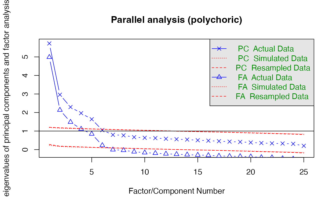

Figure 1: Parallel analysis of the 25 bfi items: observed eigenvalues compared with those of simulated/resampled random data.

Parallel analysis suggests 6 factors (and 5 components).

When the data disagree with theory

The questionnaire was designed to measure five traits. If parallel analysis suggests a different number (with large samples it often suggests six for these items — the psych documentation notes that the suggested number for bfi grows with sample size), what should you do?

1. Remember what parallel analysis is: a rule of thumb, not a test of the true number. With large \(n\), random eigenvalues get very close to 1, so even small “minor” factors (e.g. two items with similar wording) pass the threshold.
2. Fit both solutions (5 and 6 factors) and compare them: is the extra factor interpretable? Does it have at least three items with substantial loadings, or is it a “doublet” of two items? Does it split a known trait into two meaningful facets?
3. Choose the solution you can defend on theoretical and empirical grounds, and report what the alternatives looked like.

For the Big Five, the theory is strong and the sixth factor (if any) tends to be a small one, so we continue with five factors — and you will look at the six-factor solution in Exercise 4.

7. Fitting the model

fa5 <- fa(bfi_items,
          nfactors = 5,
          fm       = "minres",     # minimum residual extraction
          rotate   = "oblimin",    # oblique rotation: factors may correlate
          cor      = "poly")       # polychoric correlations

Why an oblique rotation?

The raw (“unrotated”) solution is mathematically valid but hard to interpret. Rotation turns the factor axes to obtain simple structure: each item loads strongly on one factor and weakly on the others.

• Orthogonal rotations (e.g. "varimax") force factors to be uncorrelated.
• Oblique rotations (e.g. "oblimin", "promax") allow correlations between factors.

Personality traits are correlated in real people (e.g. emotional stability and conscientiousness). Forcing them to be uncorrelated distorts the loadings. An oblique rotation lets the data decide: if the factors are in fact uncorrelated, oblimin will return nearly the same solution as varimax. So oblique rotation is the sensible default for psychological traits.

Loadings

print(fa5$loadings, cutoff = 0.3, sort = TRUE)

#> 
#> Loadings:
#>    MR2    MR3    MR4    MR1    MR5   
#> N1  0.865                            
#> N2  0.811                            
#> N3  0.739                            
#> N4  0.502 -0.408                     
#> N5  0.517                            
#> E1        -0.589                     
#> E2        -0.703                     
#> E4         0.631                     
#> C1                0.588              
#> C2                0.705              
#> C3                0.606              
#> C4               -0.688              
#> C5               -0.598              
#> A2                       0.704       
#> A3                       0.704       
#> A5                       0.564       
#> O1                              0.573
#> O2                             -0.503
#> O3                              0.660
#> O5                             -0.593
#> A1                      -0.496       
#> A4                       0.474       
#> E3         0.437                0.322
#> E5         0.448                     
#> O4        -0.368                0.445
#> 
#>                  MR2   MR3   MR4   MR1   MR5
#> SS loadings    2.752 2.224 2.241 2.132 1.876
#> Proportion Var 0.110 0.089 0.090 0.085 0.075
#> Cumulative Var 0.110 0.199 0.289 0.374 0.449

psych names factors after the extraction method — MR1, MR2, … for minres, ML1, ML2, … for maximum likelihood, PA1, … for principal axis — and orders them by the variance they explain, so the numbers do not follow the order A, C, E, N, O. Let’s find out which trait each factor represents by checking which group of items loads most on it:

L <- unclass(fa5$loadings)
trait <- substr(rownames(L), 1, 1)          # "A", "C", "E", "N", "O"
factor_trait <- apply(abs(L), 2, \(l) names(which.max(tapply(l, trait, mean))))
factor_trait

#> MR2 MR3 MR4 MR1 MR5 
#> "N" "E" "C" "A" "O"

TipHow to read the loadings

• Each number is a pattern loading: the direct effect of the factor on the item, controlling for the other factors. Loadings below 0.3 in absolute value are hidden to reveal the structure.
• Each factor collects the items of one trait: MR2 = N, MR3 = E, MR4 = C, MR1 = A, MR5 = O.
• Negative loadings belong to reverse-keyed items (e.g. A1, C4, C5, E1, E2): they are not a problem, they show that the item measures the opposite pole.
• An item with two loadings above 0.3 is a cross-loading item: it is less clean as a measure of one trait.

Communalities and uniquenesses

data.frame(h2 = round(fa5$communality, 2),
           u2 = round(fa5$uniquenesses, 2)) |>
  arrange(h2) |>
  head(5)

#>      h2   u2
#> A1 0.26 0.74
#> O2 0.30 0.70
#> A4 0.35 0.65
#> O4 0.35 0.65
#> C3 0.36 0.64

The mean communality is 0.48: on average the five factors explain about 48% of the variance of an item. This is typical for single personality items, which contain a lot of item-specific variance and noise. Items with very low \(h^2\) are weakly related to the factors.

Factor correlations

Phi <- fa5$Phi
dimnames(Phi) <- list(factor_trait, factor_trait)
round(Phi, 2)

#>       N     E     C     A    O
#> N  1.00 -0.21 -0.19 -0.06 0.01
#> E -0.21  1.00  0.25  0.32 0.15
#> C -0.19  0.25  1.00  0.22 0.21
#> A -0.06  0.32  0.22  1.00 0.20
#> O  0.01  0.15  0.21  0.20 1.00

The factor correlation matrix \(\Phi\) exists only for oblique rotations. The largest correlation (in absolute value) is 0.32. These correlations are moderate rather than zero — which is precisely why an orthogonal rotation would be a poor fit to the theory.

8. How well does the model fit?

c(TLI   = fa5$TLI,
  RMSEA = unname(fa5$RMSEA[1]),
  RMSR  = fa5$rms)

#>     TLI   RMSEA    RMSR 
#> 0.85567 0.06729 0.03008

TipHow to read the fit indices

Conventional guidelines (e.g. Hu & Bentler, 1999), to be used cautiously — they were developed for confirmatory models with continuous data and are rough guides in exploratory analysis:

Index	Measures	Commonly read as acceptable	Good
RMSEA (root mean square error of approximation)	misfit per degree of freedom	< 0.08	< 0.06 (≤ 0.05 “close”)
TLI (Tucker–Lewis index) and CFI (comparative fit index)	improvement over a null model of no correlations	≥ 0.90	≥ 0.95
RMSR (root mean square residual)	average residual correlation	< 0.08	< 0.05

Here TLI = 0.86 and RMSEA = 0.067. psych does not report CFI for fa(); it is standard output of confirmatory factor analysis software such as lavaan. With polychoric correlations these indices are only approximate. Here TLI is below the 0.90 guideline. Exploratory models of single personality items often fit only moderately, because items have many small secondary associations (similar wording, minor facets) that a five-factor model does not capture; judge fit together with interpretability and residuals, not by a single cut-off.

To compare, fit the same model with an orthogonal rotation and maximum likelihood:

fa5_ml_vmx <- fa(bfi_items, nfactors = 5, fm = "ml",
                 rotate = "varimax", cor = "poly")
colnames(fa5_ml_vmx$loadings)               # ML1, ML2, ... for maximum likelihood

#> [1] "ML1" "ML2" "ML3" "ML5" "ML4"

The fit indices of an orthogonal and an oblique rotation of the same extraction are identical — rotation does not change how well the model reproduces the correlations, only how the factors are described. What changes is interpretability and whether factor correlations are allowed.

9. Factor scores

Each person’s estimated position on each factor:

scores <- fa5$scores
colnames(scores) <- factor_trait[colnames(scores)]
head(round(scores, 2), 3)

#>           N    E     C     A     O
#> 61617 -0.20 0.06 -1.46 -0.95 -1.79
#> 61618  0.14 0.48 -0.64 -0.06 -0.29
#> 61620  0.66 0.16 -0.07 -0.68  0.22

Factor scores are estimates (several methods exist; the default is “regression”). They are useful for exploration, but in research it is common to use simple sum or mean scores of the items of each scale (after reversing the reverse-keyed items), or to model the latent variables directly in a structural equation model.

10. Reliability: Cronbach’s α and McDonald’s ω

Once you know which items form a scale, check its internal consistency — how consistently the items measure the same thing.

consc <- bfi_items[, paste0("C", 1:5)]
alpha_c <- psych::alpha(consc, keys = c("C4", "C5"))   # reverse C4 and C5
alpha_c$total[, c("raw_alpha", "std.alpha", "average_r")]

#>  raw_alpha std.alpha average_r
#>     0.7373    0.7409    0.3638

The keys argument tells alpha() which items to reverse before combining them. Forgetting it makes α artificially low (or even negative), because reverse-keyed items then pull in the opposite direction; psych warns you if some items correlate negatively with the total.

Cronbach’s α = 0.74. Values around 0.7–0.8 are usually considered adequate for research scales. α assumes that all items load equally on the factor (tau-equivalence); when loadings differ, it underestimates reliability. McDonald’s ω total uses the factor loadings and does not need this assumption:

omega_c <- psych::omega(consc, nfactors = 1, key = c(1, 1, 1, -1, -1),
                        plot = FALSE)
omega_c$omega.tot

#> [1] 0.742

ω total is 0.74. (With one factor, ω hierarchical is not meaningful and psych tells you so; for multi-factor questionnaires, omega() with 3 or more group factors also reports ω hierarchical, the share of variance due to a general factor.)

WarningCommon pitfalls

1. Using varimax for traits that are expected to correlate. Prefer an oblique rotation (oblimin); it reduces to an orthogonal solution if the factors are in fact uncorrelated.
2. Pearson correlations on few-category Likert items. They attenuate correlations; use cor = "poly".
3. Letting one rule decide the number of factors. Parallel analysis, scree, theory and interpretability should be weighed together — and alternatives reported.
4. Applying fit-index cut-offs mechanically (or using invented ones such as “TLI > 0.88 is excellent”). Use conventional guides (RMSEA < .06–.08, TLI/CFI ≥ .90–.95) with caution.
5. Forgetting reverse-keyed items when computing α or sum scores.
6. Calling PCA “factor analysis”. PCA summarises total variance; FA models common variance with an explicit error term.

11. Check your understanding

NoteQ1. An item has communality 0.25. What is its uniqueness, and what does it mean?

Uniqueness = 1 − 0.25 = 0.75: three quarters of the item’s variance is not explained by the common factors (it is item-specific variance or measurement error).

NoteQ2. Does changing the rotation from varimax to oblimin change TLI and RMSEA?

No. Rotation re-expresses the same fitted model; the reproduced correlation matrix — and so the fit — is the same. It changes the loadings and whether factors may correlate.

NoteQ3. Why can PCA loadings look “better” (larger) than FA loadings on the same data?

PCA explains total variance, including each item’s unique noise, so components absorb error and loadings are inflated. FA separates common from unique variance.

NoteQ4. Item E1 has a loading of −0.55 on the Extraversion factor. Is it a bad item?

Not necessarily: E1 (“Don’t talk a lot”) is reverse-keyed. Its negative loading means it measures introversion, the opposite pole of the factor, as intended.

12. Exercises

★ Exercise 1 — one factor in base R. Using the simulated items from section 2, (a) compute the communalities from factanal() (hint: 1 - fa_1$uniquenesses) and compare them with the squared true loadings; (b) explain in one sentence why item 5 has the smallest communality.

TipSolution

data.frame(true_h2 = true_load^2,
           estimated_h2 = round(1 - fa_1$uniquenesses, 2))

The estimates are close to 0.64, 0.49, 0.36, 0.25, 0.16 (sampling error makes them differ slightly). Item 5 has the weakest true loading (0.4), so only 16% of its variance comes from the factor; the rest is noise.

★ Exercise 2 — predict. You fit fa(bfi_items, 5, rotate = "varimax", cor = "poly") and fa(bfi_items, 5, rotate = "oblimin", cor = "poly"). Without running: (a) which output contains a factor correlation matrix Phi? (b) will the two TLI values differ? (c) will the loadings differ?

TipSolution

1. Only the oblimin solution (varimax factors are uncorrelated by construction). (b) No — same extraction, same fit. (c) Yes, somewhat: oblimin loadings are cleaner when factors truly correlate, because the varimax solution must express shared variance between traits as cross-loadings.

★★ Exercise 3 — debug the reliability. A student computes the reliability of the Agreeableness scale and gets a surprisingly low α with a warning about negatively correlated items:

psych::alpha(bfi_items[, paste0("A", 1:5)])

Explain the problem and fix it.

TipSolution

A1 (“Am indifferent to the feelings of others”) is reverse-keyed and correlates negatively with the other items. Reverse it:

psych::alpha(bfi_items[, paste0("A", 1:5)], keys = "A1")

α increases noticeably once A1 is scored in the right direction. (check.keys = TRUE would reverse it automatically, but specifying the keys from the questionnaire’s documentation is safer.)

★★ Exercise 4 — five or six? Fit a six-factor solution (fm = "minres", rotate = "oblimin", cor = "poly"). Print the loadings with cutoff = 0.3. Which items load on the sixth factor? Is it a meaningful trait, a facet of an existing trait, or a minor factor? Which solution would you report, and why?

TipSolution

fa6 <- fa(bfi_items, nfactors = 6, fm = "minres",
          rotate = "oblimin", cor = "poly")
print(fa6$loadings, cutoff = 0.3, sort = TRUE)
c(TLI5 = fa5$TLI, TLI6 = fa6$TLI)

Fit always improves a little with more factors. Look at the extra factor: typically it has only a few items with modest loadings (often a subset of Openness or Extraversion items), and most of the five-factor structure is unchanged. If the sixth factor is weak, has fewer than three salient items and lacks a clear theoretical meaning, the five-factor solution is easier to defend — but report that parallel analysis suggested six and what the sixth factor looked like.

★★★ Exercise 5 — mini-analysis on a short scale. Take only the 10 Neuroticism and Extraversion items (N1–N5, E1–E5). (a) Run a parallel analysis with polychoric correlations. (b) Fit a two-factor oblique solution and interpret the loadings. (c) What is the correlation between the two factors? (d) Compute α for each scale (remember the reverse-keyed E1 and E2).

TipSolution

ne <- bfi_items[, c(paste0("N", 1:5), paste0("E", 1:5))]

set.seed(1)
fa.parallel(ne, fa = "fa", cor = "poly", n.iter = 20)

fa2 <- fa(ne, nfactors = 2, fm = "minres", rotate = "oblimin",
          cor = "poly")
print(fa2$loadings, cutoff = 0.3)
round(fa2$Phi, 2)

psych::alpha(ne[, paste0("N", 1:5)])$total$raw_alpha
psych::alpha(ne[, paste0("E", 1:5)], keys = c("E1", "E2"))$total$raw_alpha

The N items load on one factor and the E items on the other, with E1 and E2 negative. The two factors are only weakly correlated (check the sign and size in Phi). Both scales typically have α above 0.75. Parallel analysis usually suggests two factors, possibly more with this large sample.

Summary

Idea / function	What it does
\(X = \Lambda F + \varepsilon\)	items = loadings × latent factors + unique part
polychoric(x)$rho	correlations for ordinal (Likert) items
KMO(), cortest.bartlett()	factorability checks
fa.parallel(x, cor = "poly")	parallel analysis for the number of factors
fa(x, nfactors, fm = "minres", rotate = "oblimin", cor = "poly")	exploratory factor analysis
$loadings, $communality, $uniquenesses, $Phi	pattern loadings, \(h^2\), \(u^2\), factor correlations
$TLI, $RMSEA, $rms	fit indices
alpha(x, keys = ), omega(x)	reliability (α, ω), with reverse-keyed items

• FA explains common variance through latent factors; PCA summarises total variance.
• Use polychoric correlations for Likert items and an oblique rotation for traits that may correlate.
• Decide the number of factors with parallel analysis and theory, and report alternatives.
• Read fit indices with conventional, cautious thresholds; rotation does not change fit.
• Check reliability with α and ω, after reversing reverse-keyed items.

NoteFurther reading

• Revelle, W., An introduction to psychometric theory with applications in R, https://personality-project.org/r/book/
• Revelle, W. & Condon, D. M. (2019), “Reliability from α to ω: A tutorial”, preprint https://osf.io/preprints/psyarxiv/2y3w9
• psych package documentation for fa(), https://search.r-project.org/CRAN/refmans/psych/html/fa.html