library(tidymodels)
library(ranger) # engine for random forestsRandom forests
Many unstable trees, averaged, make one stable predictor
Bagging and random feature subsetting, out-of-bag error, tuning mtry and min_n with tidymodels and ranger, permutation versus impurity importance (and their biases), and partial dependence plots.
NoteLearning objectives
By the end of this lesson you will be able to:
- explain bagging as averaging trees grown on bootstrap samples, and why averaging reduces variance;
- explain how random feature subsetting (
mtry) decorrelates the trees; - use and correctly interpret the out-of-bag (OOB) error;
- tune a random forest with
rand_forest()+rangerin tidymodels; - compare permutation and impurity importance, know their biases, and draw a partial dependence plot.
1. Why a forest?
At the end of the decision-tree lesson we saw that trees fitted to slightly different samples of the same data can look very different and give very different predictions: trees have low bias but high variance.
Think of estimating the weight of an ox at a country fair. Any single guess is noisy; the average of many independent guesses is often remarkably close to the truth, because the individual errors partly cancel. A random forest applies the same idea to trees: grow many different trees and average their predictions (or let them vote).
We use the same Titanic preparation as in the ML workflow lesson:
titanic <- readr::read_csv(data_path("titanic_data.csv"),
                           na = c("", "NA", "?"), show_col_types = FALSE) |>
  select(survived, pclass, sex, age, sibsp, parch, fare, embarked) |>
  mutate(
    survived = factor(survived, levels = c(1, 0), labels = c("yes", "no")),
    pclass   = factor(pclass, levels = 1:3, labels = c("1st", "2nd", "3rd")),
    sex      = factor(sex),
    embarked = factor(embarked)
  )

set.seed(2026)
titanic_split <- initial_split(titanic, prop = 0.75, strata = survived)
titanic_train <- training(titanic_split)
titanic_test  <- testing(titanic_split)
set.seed(2026)
titanic_folds <- vfold_cv(titanic_train, v = 5, strata = survived)
titanic_metrics <- metric_set(roc_auc, accuracy, sensitivity, specificity,
                              brier_class, mn_log_loss)
2. Bagging: bootstrap + aggregate
Bagging (bootstrap aggregating, Breiman 1996) works like this:
- Draw \(B\) bootstrap samples of the training data (same size, with replacement — as in the bootstrap lesson).
- Grow a large, unpruned tree on each.
- Predict by averaging: the mean for regression, the average class probability (or the majority vote) for classification.
Unpruned trees have low bias but high variance; averaging keeps the low bias and reduces the variance.
How much does averaging help?
If the \(B\) predictions each have variance \(\sigma^2\) and were independent, their average would have variance \(\sigma^2 / B\). But the trees are grown on overlapping samples from the same data, so they are correlated. With pairwise correlation \(\rho\):
\[ \operatorname{Var}\Big(\frac1B\sum_{b=1}^B T_b\Big) = \rho\,\sigma^2 + \frac{1-\rho}{B}\,\sigma^2 . \]
var_avg <- function(rho, B, sigma2 = 1) rho * sigma2 + (1 - rho) * sigma2 / B
outer(c(rho_0 = 0, rho_0.3 = 0.3, rho_0.7 = 0.7), c(1, 10, 100, 1000),
      var_avg)
#> [,1] [,2] [,3] [,4]
#> rho_0 1 0.10 0.010 0.0010
#> rho_0.3 1 0.37 0.307 0.3007
#> rho_0.7 1 0.73 0.703 0.7003Let us check the formula by simulation, with \(B = 50\) correlated “trees” and \(\rho = 0.3\):
set.seed(46)
B <- 50
rho <- 0.3
sims <- replicate(5000, {
  common <- rnorm(1)                 # the part shared by all trees
  own <- rnorm(B)                    # the part specific to each tree
  mean(sqrt(rho) * common + sqrt(1 - rho) * own)
})
c(simulated = var(sims), formula = var_avg(rho, B))
#> simulated formula
#> 0.3124 0.3140
TipHow to read this output
- As \(B\) grows, the second term vanishes, but the first (\(\rho\sigma^2\)) does not. With \(\rho = 0.7\), even 1000 trees only reduce the variance to 70% of a single tree’s.
- So adding trees never hurts (it does not cause overfitting), but beyond a few hundred it barely helps. To do better, we must make the trees less correlated.
3. Random forests: decorrelating the trees
If one predictor is very strong (on the Titanic, sex), almost every bagged tree will split on it first, and the trees will be similar. Random forests (Breiman 2001) add one twist: at each split, only a random subset of mtry predictors is considered as candidates.
mtry= number of predictors \(p\) → plain bagging.- Small
mtry→ trees are forced to explore other variables → lower correlation \(\rho\), at the price of slightly worse individual trees. - Common defaults: \(\lfloor\sqrt p\rfloor\) for classification and \(\lfloor p/3 \rfloor\) for regression (the
randomForestpackage);rangeruses \(\lfloor\sqrt p\rfloor\) for both. With our 7 predictors, the classification default is 2.
The other main tuning parameter is the minimum node size (min_n in tidymodels, min.node.size in ranger): nodes smaller than this are not split. Larger values give smaller, smoother trees. The number of trees is not really a tuning parameter: use “enough” (a few hundred to a thousand) and check that results are stable.
4. Out-of-bag (OOB) error
Each bootstrap sample leaves out some observations. The probability that a given observation is not drawn in a sample of size \(n\) is \((1 - 1/n)^n \approx e^{-1} \approx 0.368\):
set.seed(46)
n <- 1000
in_bag <- replicate(500, length(unique(sample(n, replace = TRUE))) / n)
c(simulated = mean(1 - in_bag), exact = (1 - 1 / n)^n, limit = exp(-1))
#> simulated exact limit
#> 0.3673 0.3677 0.3679So every observation is out of bag for roughly a third of the trees. Predicting each observation using only those trees gives an OOB prediction for every training row, and from those an OOB error — essentially for free, without a separate validation set.
To look at it, we prepare the training data with a recipe (impute missing values; forests need no dummies or scaling) and call ranger() directly:
rf_rec <- recipe(survived ~ ., data = titanic_train) |>
  step_impute_median(all_numeric_predictors()) |>
  step_impute_mode(all_nominal_predictors())

train_baked <- rf_rec |> prep() |> bake(new_data = NULL)
oob_curve <- tibble(trees = c(10, 25, 50, 100, 250, 500, 1000, 2000)) |>
mutate(oob_brier = map_dbl(trees, \(b) {
ranger(survived ~ ., data = train_baked, num.trees = b,
probability = TRUE, seed = 46)$prediction.error
}))
ggplot(oob_curve, aes(trees, oob_brier)) +
geom_line(linewidth = 1) +
geom_point() +
scale_x_log10() +
labs(x = "Number of trees (log scale)", y = "OOB Brier score")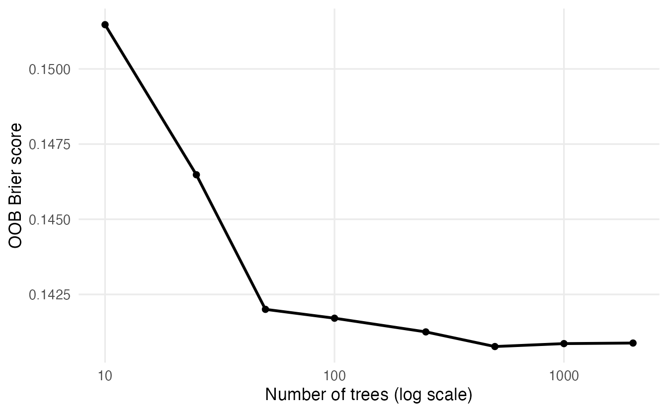
For a probability forest (probability = TRUE, which tidymodels uses for classification) prediction.error is the OOB Brier score; for a class-vote forest it is the OOB misclassification rate.
5. Tuning a forest with tidymodels
rf_spec <- rand_forest(mtry = tune(), min_n = tune(), trees = 1000) |>
  set_engine("ranger", importance = "permutation") |>
  set_mode("classification")

rf_wf <- workflow() |>
  add_recipe(rf_rec) |>
  add_model(rf_spec)
importance = "permutation" is an engine argument passed to ranger(); it asks ranger to compute permutation importance (section 6) during fitting.
mtry must be an integer between 1 and the number of predictors (7 here). We build the grid explicitly so that this is guaranteed:
rf_grid <- grid_regular(mtry(range = c(1L, 7L)),
                        min_n(range = c(2L, 30L)),
                        levels = c(7, 3))
rf_grid |> count(min_n)
#> # A tibble: 3 × 2
#> min_n n
#> <int> <int>
#> 1 2 7
#> 2 16 7
#> 3 30 7set.seed(2026)
rf_res <- tune_grid(rf_wf, resamples = titanic_folds, grid = rf_grid,
metrics = titanic_metrics)This fits 21 × 5 = 105 forests of 1000 trees each — about a minute or two on a laptop. For larger data, use fewer grid points or a racing method (lesson 47).
autoplot(rf_res, metric = "roc_auc")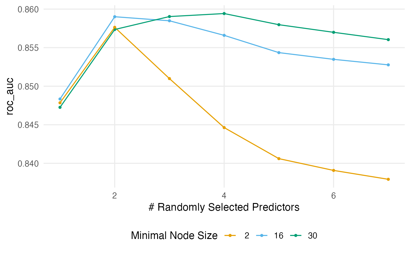
show_best(rf_res, metric = "roc_auc", n = 5)#> # A tibble: 5 × 8
#> mtry min_n .metric .estimator mean n std_err .config
#> <int> <int> <chr> <chr> <dbl> <int> <dbl> <chr>
#> 1 4 30 roc_auc binary 0.8594 5 0.01174 pre0_mod12_post0
#> 2 3 30 roc_auc binary 0.8590 5 0.01171 pre0_mod09_post0
#> 3 2 16 roc_auc binary 0.8590 5 0.01307 pre0_mod05_post0
#> 4 3 16 roc_auc binary 0.8585 5 0.01223 pre0_mod08_post0
#> 5 5 30 roc_auc binary 0.8580 5 0.01192 pre0_mod15_post0best_rf <- select_best(rf_res, metric = "roc_auc")
best_rf#> # A tibble: 1 × 3
#> mtry min_n .config
#> <int> <int> <chr>
#> 1 4 30 pre0_mod12_post0
TipHow to read this output
- Look at the shape of the curves rather than at the single best point: forests are usually not very sensitive to their tuning parameters, and many combinations are within one standard error of the best.
- Compare the right end of each curve (
mtry = 7, bagging) with the smaller values: if smallermtryis better, decorrelating the trees helped. - The best combination here is
mtry= 4 andmin_n= 30.
rf_final <- rf_wf |>
  finalize_workflow(best_rf) |>
  last_fit(titanic_split, metrics = titanic_metrics)
collect_metrics(rf_final)
#> # A tibble: 6 × 4
#> .metric .estimator .estimate .config
#> <chr> <chr> <dbl> <chr>
#> 1 accuracy binary 0.8415 pre0_mod0_post0
#> 2 sensitivity binary 0.728 pre0_mod0_post0
#> 3 specificity binary 0.9113 pre0_mod0_post0
#> 4 roc_auc binary 0.8767 pre0_mod0_post0
#> 5 brier_class binary 0.1268 pre0_mod0_post0
#> 6 mn_log_loss binary 0.4130 pre0_mod0_post06. Variable importance
A forest of 1000 trees cannot be read like a single tree. Variable importance measures summarise how much each predictor contributes. There are two very different kinds.
| Impurity importance (mean decrease in Gini / “MDI”) | Permutation importance (mean decrease in accuracy / “MDA”) | |
|---|---|---|
| Idea | Sum, over all splits on the variable, of the impurity decrease they achieve | Shuffle the variable’s values (breaking its link with \(y\)) and measure how much the error increases |
| Computed on | The training (in-bag) data | Out-of-bag (or test) data |
| Cost | Free | Requires extra predictions |
| Main bias | Favours variables with many possible split points (continuous variables, factors with many levels), even if they are pure noise | With correlated predictors, shuffling one creates unrealistic combinations; importance can be shared or inflated |
| ranger | importance = "impurity" (or "impurity_corrected") |
importance = "permutation" |
| randomForest | importance(fit, type = 2) — MeanDecreaseGini |
importance(fit, type = 1) — MeanDecreaseAccuracy (classification) or %IncMSE (regression) |
(The old version of this lesson had the last row swapped: in randomForest, type = 1 is the permutation measure and type = 2 the impurity measure; %IncMSE exists only for regression forests.)
The bias of impurity importance, demonstrated
Add two variables of pure noise to the training data — one continuous (many split points) and one binary — and compare the two importance measures:
set.seed(46)
train_noise <- train_baked |>
  mutate(noise_cont = rnorm(n()),
         noise_bin = factor(sample(c("a", "b"), n(), replace = TRUE)))

imp_compare <- map(c("impurity", "permutation"), \(type) {
  fit <- ranger(survived ~ ., data = train_noise, num.trees = 500,
                importance = type, seed = 46)
  imp <- fit$variable.importance
  tibble(variable = names(imp), importance = imp / max(imp), type = type)
}) |>
list_rbind()ggplot(imp_compare,
aes(importance, reorder(variable, importance), fill = type)) +
geom_col(position = "dodge") +
labs(x = "Importance (relative to the top variable)", y = NULL, fill = NULL)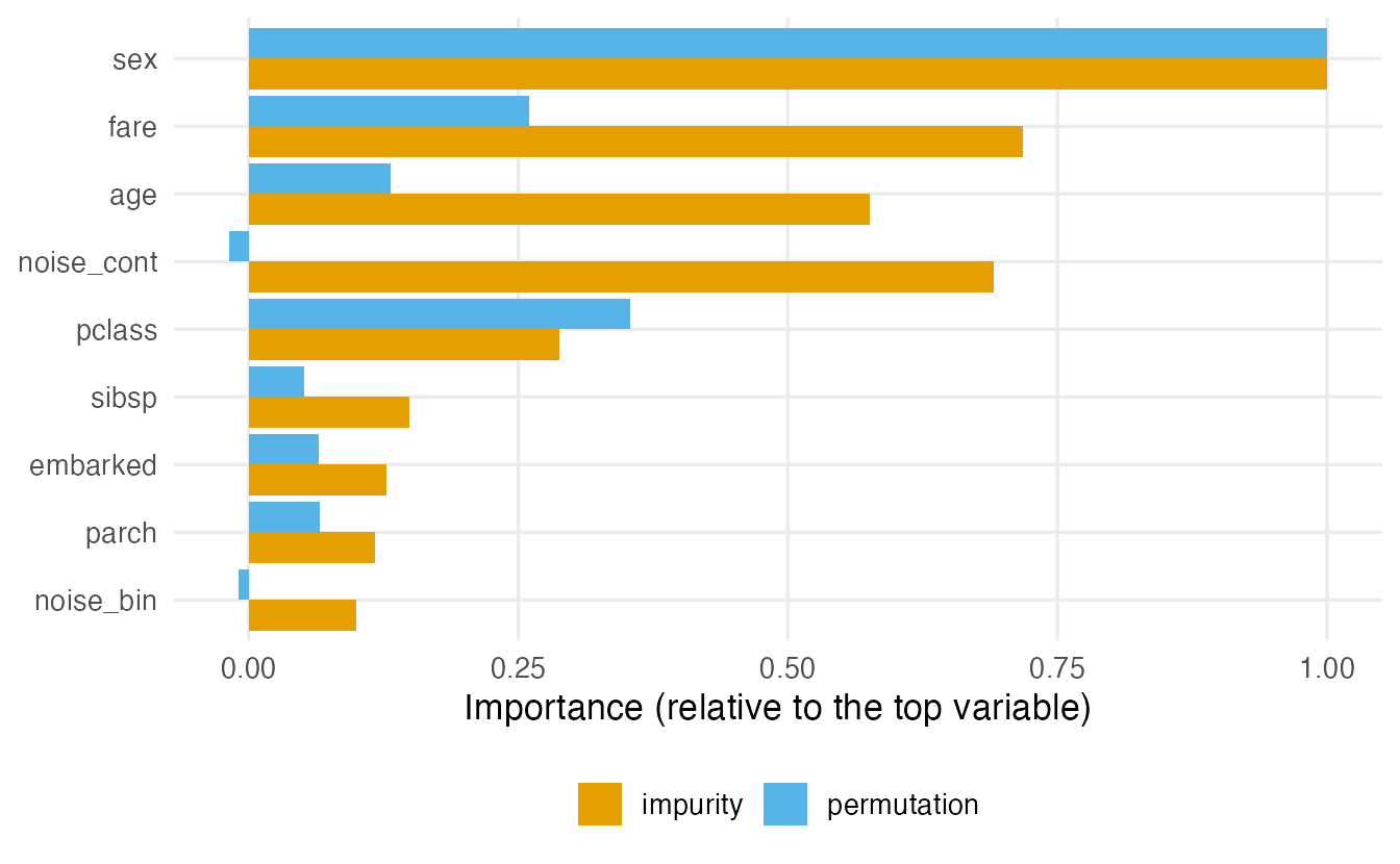
imp_compare |>
  group_by(type) |>
  mutate(rank = rank(-importance)) |>
  filter(startsWith(variable, "noise")) |>
  select(type, variable, importance, rank)
#> # A tibble: 4 × 4
#> # Groups: type [2]
#> type variable importance rank
#> <chr> <chr> <dbl> <dbl>
#> 1 impurity noise_cont 0.6908 3
#> 2 impurity noise_bin 0.09928 9
#> 3 permutation noise_cont -0.01848 9
#> 4 permutation noise_bin -0.009655 8The continuous noise variable noise_cont receives a sizeable impurity importance — it offers hundreds of possible split points, and deep trees use some of them to fit noise in the training data — while its permutation importance is close to zero (it can even be slightly negative, which just means “no effect”). The binary noise variable is near zero for both. Real continuous variables such as age and fare benefit from the same bias under impurity importance. Prefer permutation importance for interpretation, and remember it is a property of the model, not a causal effect.
Importance of the tuned forest
rf_final |>
  extract_fit_parsnip() |>
  plot_importance(n = 7)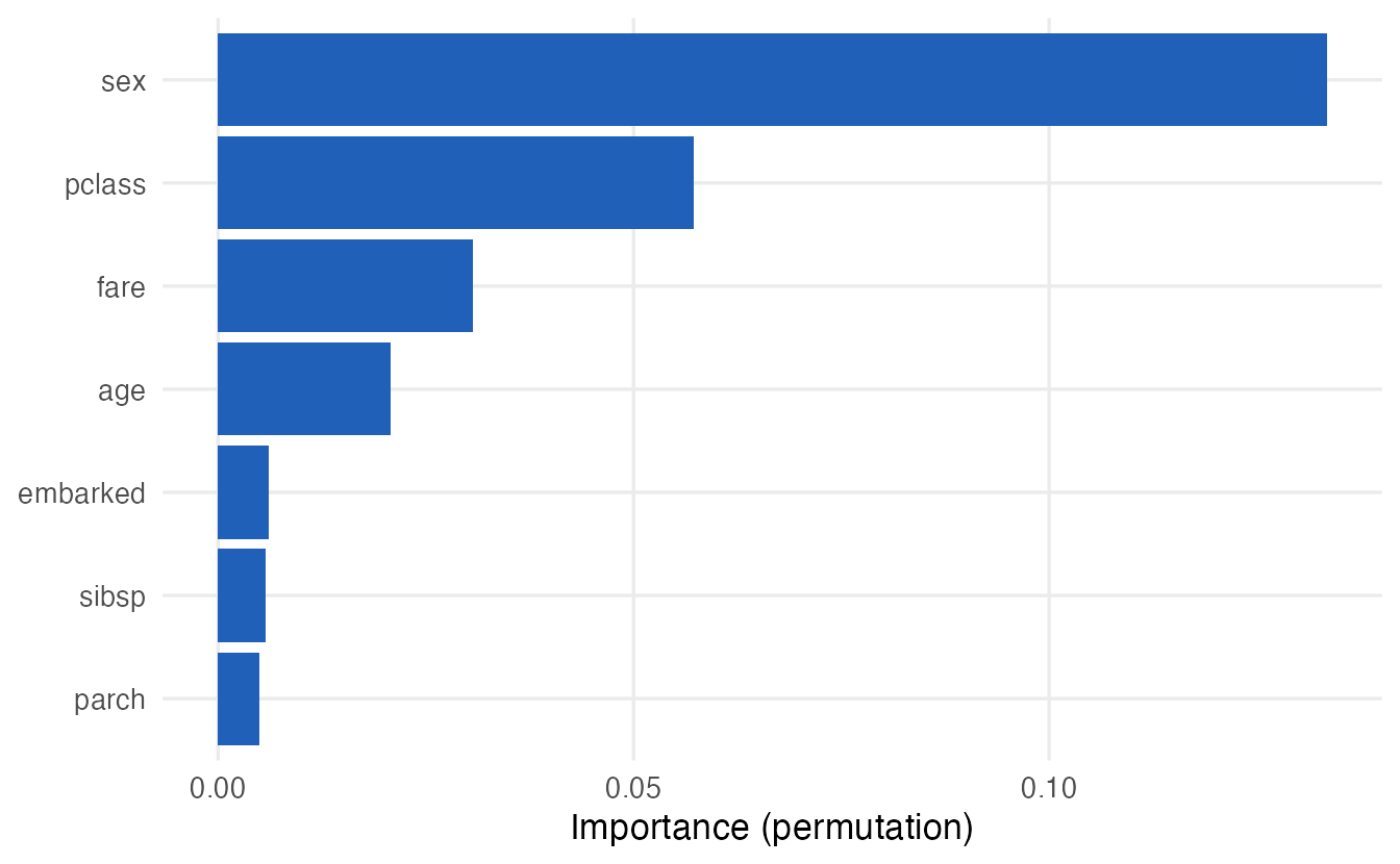
7. Partial dependence: how does a variable matter?
Importance says how much a variable matters, not in which direction. A partial dependence (PD) curve shows how the average prediction changes as one variable varies, holding the distribution of the others fixed. It is simple enough to compute by hand:
- Choose a grid of values for the variable (e.g. ages 1, 3, …, 75).
- For each value \(v\): set the variable to \(v\) for every passenger in the training data, predict, and average the predicted probabilities.
rf_fitted_wf <- extract_workflow(rf_final)
age_grid <- seq(1, 75, by = 2)

pd_age <- tibble(age = age_grid) |>
  mutate(prob_yes = map_dbl(age, \(a) {
    new <- titanic_train |> mutate(age = a)
    mean(predict(rf_fitted_wf, new_data = new, type = "prob")$.pred_yes)
}))ggplot(pd_age, aes(age, prob_yes)) +
geom_line(linewidth = 1) +
labs(x = "Age (years)", y = "Average predicted P(survival)")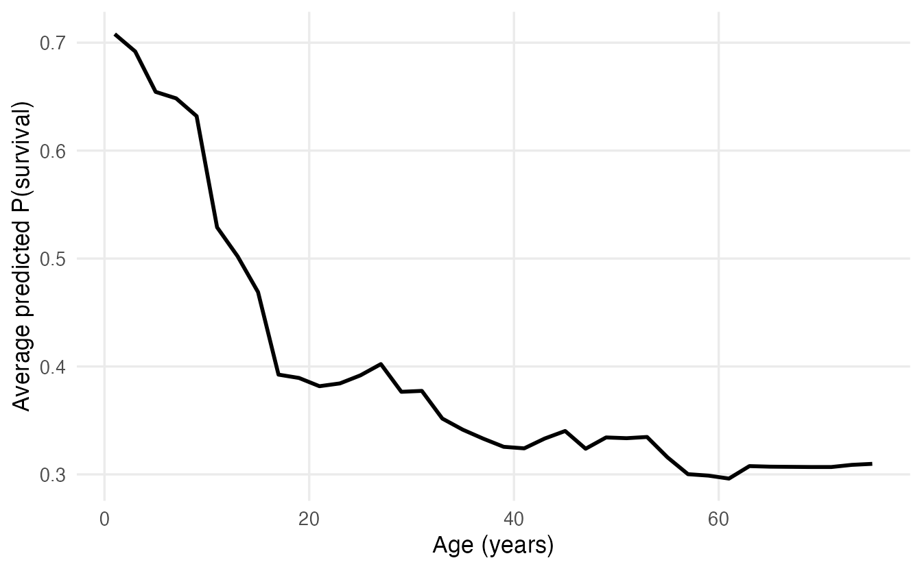
Because we predict with the whole workflow, the recipe (imputation) is applied automatically to the modified data. The curve typically shows a higher survival probability for young children, consistent with “women and children first”. A PD curve is an average: if age acts differently for men and women (an interaction), compute separate curves by sex (Exercise 4). Packages such as DALEX and pdp automate this and add individual (ICE) curves.
NoteGoing deeper: partial dependence formally
For a fitted model \(\hat f\) and a variable \(x_S\) with the remaining variables \(x_C\), the partial dependence function is estimated by \[ \hat f_S(v) = \frac1n \sum_{i=1}^n \hat f(v, x_{C,i}) . \] It is an average over the marginal distribution of \(x_C\). When \(x_S\) is strongly correlated with some \(x_C\), this average includes unrealistic combinations (a 2-year-old travelling alone in 1st class with 5 siblings), so PD curves can be misleading; accumulated local effects (ALE) plots are an alternative designed for this case.
WarningCommon pitfalls
- Interpreting impurity importance as “the truly important variables”. It favours continuous and high-cardinality predictors, even pure noise. Use permutation importance.
- Mixing up
randomForestimportance types.type = 1is permutation (MeanDecreaseAccuracy, or%IncMSEfor regression),type = 2impurity (MeanDecreaseGini). - Non-integer
mtry(e.g.seq(2, p/2, length = 6)):mtryis a count of variables. Usemtry(range = c(1L, p)). - Thinking more trees cause overfitting. They don’t; they only cost time. Overfitting is controlled by
min_n(andmtry). - Treating OOB error as an unbiased estimate after tuning on it. Selection makes any score optimistic; keep a test set.
- Reading importance or PD as causal effects. They describe what the model uses, not what would happen if we intervened.
8. Check your understanding
9. Exercises
★ Exercise 1 — OOB by simulation. Modify the oob-fraction code for \(n = 10\) and \(n = 100\). How does the out-of-bag fraction compare with \(e^{-1}\)?
TipSolution
for (n in c(10, 100)) {
  in_bag <- replicate(5000, length(unique(sample(n, replace = TRUE))) / n)
  print(c(n = n, simulated = mean(1 - in_bag), exact = (1 - 1 / n)^n))
}
For \(n = 10\) the fraction is about 0.35, for \(n = 100\) about 0.366; it approaches \(e^{-1} \approx 0.368\) from below as \(n\) grows.
★★ Exercise 2 — bagging vs forest. Using fit_resamples() on titanic_folds, compare two forests with min_n = 5 and 500 trees: one with mtry = 7 (bagging) and one with mtry = 2. Which has the higher CV ROC AUC? Is the difference larger than the standard errors?
TipSolution
cv_forest <- function(m) {
  spec <- rand_forest(mtry = m, min_n = 5, trees = 500) |>
    set_engine("ranger") |> set_mode("classification")
  set.seed(2026)
  workflow(rf_rec, spec) |>
    fit_resamples(titanic_folds, metrics = metric_set(roc_auc)) |>
    collect_metrics() |>
    mutate(mtry = m)
}
bind_rows(cv_forest(7), cv_forest(2))
With only 7 predictors, one of which (sex) dominates, mtry = 2 usually gives a slightly higher AUC than bagging, but the difference is often of the order of one standard error. (workflow(rec, spec) is a shortcut for workflow() |> add_recipe(rec) |> add_model(spec).)
★★ Exercise 3 — impurity vs permutation on the tuned forest. Refit the final forest with importance = "impurity" and compare the ranking of the variables with the permutation ranking. Which variables move up?
TipSolution
rf_imp_spec <- rand_forest(mtry = best_rf$mtry, min_n = best_rf$min_n,
                           trees = 1000) |>
  set_engine("ranger", importance = "impurity") |>
  set_mode("classification")
set.seed(2026)
rf_imp <- workflow(rf_rec, rf_imp_spec) |> fit(titanic_train)
rf_imp |> extract_fit_parsnip() |> plot_importance(n = 7)
The continuous variables (fare, age) typically rank higher under impurity importance than under permutation importance, because they offer many split points — the bias demonstrated in section 6.
★★★ Exercise 4 — PD by sex. Compute two partial-dependence curves for age: one setting sex = "female" for everybody, one setting sex = "male". Plot them together. What does the plot suggest about an age × sex interaction?
TipSolution
pd_sex <- tidyr::expand_grid(age = age_grid, sex = c("female", "male")) |>
  mutate(prob_yes = map2_dbl(age, sex, \(a, s) {
    new <- titanic_train |>
      mutate(age = a, sex = factor(s, levels = levels(titanic$sex)))
    mean(predict(rf_fitted_wf, new_data = new, type = "prob")$.pred_yes)
  }))
ggplot(pd_sex, aes(age, prob_yes, colour = sex)) +
  geom_line(linewidth = 1) +
  labs(x = "Age", y = "Average predicted P(survival)", colour = NULL)
The female curve is much higher at all ages. If the two curves are not parallel — e.g. age matters mainly for boys, whose survival drops sharply after childhood — the forest has learned an age × sex interaction, something a logistic regression without interaction terms cannot represent.
★★ Exercise 5 — interpret. A colleague reports: “In our forest, zip_code (900 levels) is the most important variable according to MeanDecreaseGini, so location drives the outcome.” What would you check before believing this?
TipSolution
A factor with 900 levels offers an enormous number of possible splits, so impurity importance is biased in its favour, even if it carries no signal. Check its permutation importance (on OOB or test data), or the corrected impurity importance (importance = "impurity_corrected" in ranger); compare the model’s CV performance with and without the variable; and remember that importance is not causation.
Summary
| Idea / function | What it does |
|---|---|
| Bagging | Average of trees grown on bootstrap samples |
mtry |
Number of candidate predictors per split; small = decorrelated trees |
min_n |
Minimum node size; larger = smoother trees |
| OOB error | Error on observations not in each tree’s bootstrap sample (~37%) |
rand_forest(mtry, min_n, trees) \|> set_engine("ranger", importance = ...) |
tidymodels specification |
grid_regular(mtry(range = c(1L, p)), min_n(...)) |
Integer tuning grid |
| Permutation vs impurity importance | Model-based on held-out data vs free but biased to many-split variables |
plot_importance() (course helper in _common.R) |
Importance plot from the engine’s stored importance |
| Partial dependence | Average prediction as one variable varies |
- Averaging reduces variance, but only down to the shared part (\(\rho\sigma^2\)); random feature subsetting lowers \(\rho\).
- Forests need little tuning and rarely overfit by adding trees.
- OOB error is a convenient estimate, not a replacement for an untouched test set.
- Use permutation importance and partial dependence to interpret, and do not read them causally.