Model selection and validation

Choosing predictors without fooling yourself: F-tests, AIC, cross-validation

Compare nested models with F-tests, trade fit against complexity with AIC and BIC, see by simulation why stepwise selection is dangerous, and estimate prediction error honestly with train/test splits and k-fold cross-validation written by hand.

Level 4 · Models & learning ⏱ ~90 min Prerequisites: Multiple regression, Randomness and simulation

NoteLearning objectives

By the end of this lesson you will be able to:

• explain the difference between a model built to explain and a model built to predict;
• compare nested models with an F-test and any models with AIC/BIC;
• show by simulation why stepwise selection produces over-optimistic results;
• distinguish training error from test error and recognise overfitting;
• write k-fold cross-validation by hand and use it to choose between models.

library(dplyr)
library(ggplot2)
library(tidyr)

1. Why is choosing a model hard?

mtcars has 10 possible predictors of mpg. Even without interactions there are \(2^{10} = 1024\) possible subsets. Which one should we use? The answer depends on why we are building the model.

• Explanation (inference). We want to understand how \(y\) relates to particular predictors: “how much does weight matter, holding horsepower constant?”. The model should be chosen from subject-matter knowledge before looking at the results, and we care about unbiased coefficients and honest p-values and CIs.
• Prediction. We want accurate guesses of \(y\) for new observations. We do not care whether a coefficient is “significant”; we care about the error on data the model has never seen.

These goals lead to different tools. F-tests and AIC are classic tools for comparing models fitted to the same data. Cross-validation is the workhorse of prediction. And some popular practices — like letting an algorithm pick predictors and then reporting the p-values — serve neither goal well.

2. Nested models and the F-test

Two models are nested when one is a special case of the other (obtained by setting some coefficients to 0). The F-test asks: does the bigger model reduce the residual sum of squares by more than we would expect by chance?

m1 <- lm(mpg ~ wt, data = mtcars)
m2 <- lm(mpg ~ wt + hp, data = mtcars)
m3 <- lm(mpg ~ wt + hp + qsec + drat, data = mtcars)

anova(m1, m2, m3)

#> Analysis of Variance Table
#> 
#> Model 1: mpg ~ wt
#> Model 2: mpg ~ wt + hp
#> Model 3: mpg ~ wt + hp + qsec + drat
#>   Res.Df RSS Df Sum of Sq     F Pr(>F)   
#> 1     30 278                             
#> 2     29 195  1      83.3 12.91 0.0013 **
#> 3     27 174  2      20.9  1.62 0.2158   
#> ---
#> Signif. codes:  0 '***' 0.001 '**' 0.01 '*' 0.05 '.' 0.1 ' ' 1

TipHow to read this output

• Res.Df and RSS: residual degrees of freedom and residual sum of squares of each model. RSS always decreases as we add predictors.
• Row 2 compares m2 with m1: adding hp reduces the RSS by 83.3 (1 extra parameter). F = 12.4, p = 0.0015: a clear improvement.
• Row 3 compares m3 with m2: adding qsec and drat (2 parameters) reduces RSS only a little; p = 0.22. No evidence that they help.

The F-test works only for nested models fitted to the same rows. It cannot compare mpg ~ wt + hp with mpg ~ disp + qsec.

NoteGoing deeper: the F statistic

For a small model with \(\text{RSS}_0\) and \(p_0\) parameters, nested in a big one with \(\text{RSS}_1\) and \(p_1\) parameters,

\[ F = \frac{(\text{RSS}_0 - \text{RSS}_1)/(p_1 - p_0)}{\text{RSS}_1/(n - p_1)} \sim F_{p_1 - p_0,\; n - p_1} \quad \text{under } H_0 . \]

The numerator is the improvement per added parameter; the denominator is the noise level estimated from the big model.

3. AIC and BIC: fit versus complexity

Adding predictors always improves the fit to the data at hand. Information criteria add a penalty for each parameter so that extra complexity must “pay for itself”:

\[ \text{AIC} = -2\log L + 2k, \qquad \text{BIC} = -2\log L + k \log n, \]

where \(L\) is the maximised likelihood (higher = better fit), \(k\) the number of estimated parameters (including the residual variance) and \(n\) the sample size. Lower is better. They can compare non-nested models, as long as the response and the rows are the same.

AIC(m1, m2, m3)

#>    df   AIC
#> m1  3 166.0
#> m2  4 156.7
#> m3  6 157.0

BIC(m1, m2, m3)

#>    df   BIC
#> m1  3 170.4
#> m2  4 162.5
#> m3  6 165.8

Both prefer m2. The two criteria trade off differently:

• AIC aims at good prediction: it approximates how well the model would predict new data from the same population. Its penalty (2 per parameter) is mild.
• BIC aims at finding the “true” model if it is among the candidates. Its penalty (\(\log n\) per parameter, already 3.5 with \(n = 32\)) is stronger, so it picks smaller models.

Only differences in AIC matter; the absolute value means nothing. A rough guide: differences below 2 are negligible, above 10 are large.

4. Stepwise selection — and why it is dangerous

step() automates the search: starting from a model, it repeatedly adds or drops the predictor that improves AIC most, until nothing helps.

m_full <- lm(mpg ~ ., data = mtcars)
m_step <- step(m_full, direction = "both", trace = 0)
formula(m_step)

#> mpg ~ wt + qsec + am

Looks convenient. The problem is what happens after: summary(m_step) reports standard errors and p-values as if the three predictors had been chosen before seeing the data. They were not — they were chosen because they looked good in these data.

A simulation with pure noise

Let us generate a response and 40 predictors that are all pure random noise: no predictor has any relationship with y.

set.seed(2026)
n <- 100
p <- 40
noise <- as.data.frame(matrix(rnorm(n * p), nrow = n))
noise$y <- rnorm(n)

m_noise <- step(lm(y ~ ., data = noise), trace = 0)
summary(m_noise)

#> 
#> Call:
#> lm(formula = y ~ V5 + V11 + V16 + V24 + V26 + V29 + V31 + V34, 
#>     data = noise)
#> 
#> Residuals:
#>     Min      1Q  Median      3Q     Max 
#> -2.0569 -0.5871  0.0764  0.6252  2.0362 
#> 
#> Coefficients:
#>             Estimate Std. Error t value Pr(>|t|)    
#> (Intercept)   0.0529     0.1001    0.53  0.59795    
#> V5           -0.1254     0.0852   -1.47  0.14482    
#> V11          -0.1647     0.1049   -1.57  0.11973    
#> V16          -0.1898     0.1050   -1.81  0.07390 .  
#> V24           0.1473     0.0886    1.66  0.09983 .  
#> V26          -0.3897     0.0990   -3.94  0.00016 ***
#> V29          -0.1406     0.0939   -1.50  0.13785    
#> V31          -0.1345     0.0927   -1.45  0.15032    
#> V34           0.1566     0.0975    1.61  0.11159    
#> ---
#> Signif. codes:  0 '***' 0.001 '**' 0.01 '*' 0.05 '.' 0.1 ' ' 1
#> 
#> Residual standard error: 0.933 on 91 degrees of freedom
#> Multiple R-squared:  0.238,  Adjusted R-squared:  0.171 
#> F-statistic: 3.55 on 8 and 91 DF,  p-value: 0.00128

Stepwise kept 8 of the 40 noise variables. The final model has R² = 0.24 and an overall F-test p-value of 0.0013. A naive reader would conclude that the model “significantly” explains y. Every one of those relationships is fake.

How often does this happen? We repeat the experiment 20 times and count how many predictors in the selected model have p < 0.05:

set.seed(1)
n_signif <- replicate(20, {
  d <- as.data.frame(matrix(rnorm(n * p), nrow = n))
  d$y <- rnorm(n)
  sel <- step(lm(y ~ ., data = d), trace = 0)
  sum(summary(sel)$coefficients[-1, "Pr(>|t|)"] < 0.05)
})
n_signif

#>  [1]  6  2  7  3  0  4  9  7  0  5  4  2  3  2  6  2  6  9 11  5

On average 4.7 “significant” predictors per dataset, out of variables that are all noise; only 2 of the 20 runs found nothing. The p-values after selection are not valid p-values.

ImportantWhy stepwise misleads

• It runs many hidden tests and keeps the winners — a multiple-testing problem in disguise.
• The selected coefficients are biased away from zero (they were kept because they were large in this sample).
• The selection is unstable: a slightly different sample often gives a different set of predictors.

If the goal is explanation, choose the model from theory. If the goal is prediction, evaluate the whole procedure with cross-validation (Section 7), or use penalized regression, which selects and shrinks in a more stable way.

5. Overfitting: training error vs test error

To see the prediction side of the problem we simulate data where we know the truth: \(y = \sin(2\pi x) + \varepsilon\), with 30 training points. We fit polynomials of increasing degree and measure the root mean squared error (RMSE, the typical size of a prediction error) on the training data and on 1000 fresh test points from the same process.

set.seed(1)
f_true <- function(x) sin(2 * pi * x)
train <- tibble::tibble(x = runif(30), y = f_true(x) + rnorm(30, sd = 0.3))
test  <- tibble::tibble(x = runif(1000), y = f_true(x) + rnorm(1000, sd = 0.3))

rmse <- function(y, y_hat) sqrt(mean((y - y_hat)^2))

errors <- lapply(1:12, \(d) {
  fit <- lm(y ~ poly(x, d), data = train)
  tibble::tibble(degree = d,
                 train = rmse(train$y, fitted(fit)),
                 test = rmse(test$y, predict(fit, newdata = test)))
}) |>
  bind_rows()

errors |>
  pivot_longer(c(train, test), names_to = "data", values_to = "rmse") |>
  ggplot(aes(degree, rmse, colour = data)) +
  geom_hline(yintercept = 0.3, linetype = 2) +
  geom_line(linewidth = 1) +
  geom_point() +
  scale_x_continuous(breaks = 1:12) +
  labs(x = "Polynomial degree (model complexity)", y = "RMSE", colour = NULL)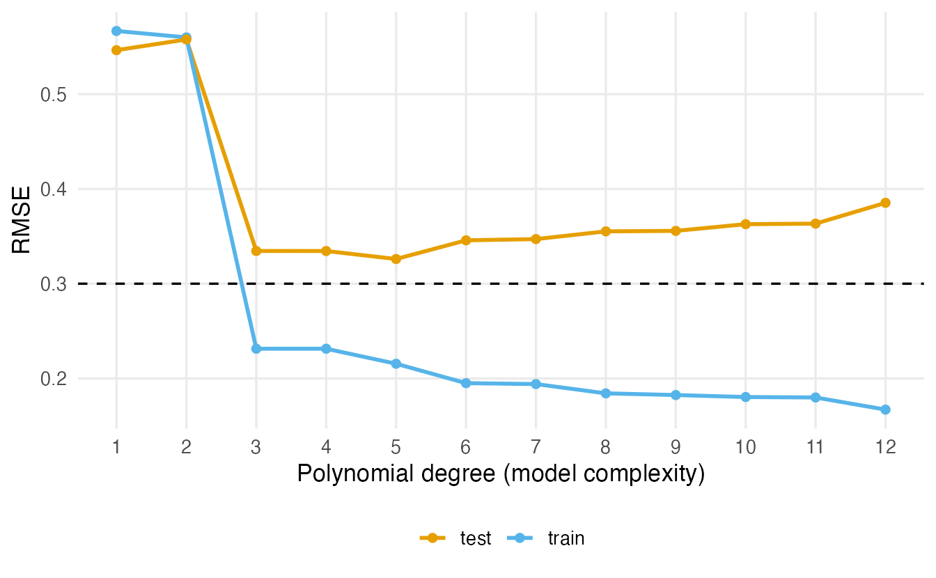

Figure 1: Training RMSE keeps falling as the polynomial degree grows; test RMSE falls, then rises again. The dashed line is the noise level (0.3), the best error any model could achieve.

This is overfitting: beyond a certain complexity, the model starts fitting the noise of the training sample. The training error keeps improving, but the error on new data gets worse. The training error is therefore a biased (optimistic) estimate of how the model will perform. The gap between the curves is the price of complexity — the bias–variance trade-off you will meet again in The machine learning workflow.

grid <- tibble::tibble(x = seq(0, 1, length.out = 300))
fits <- lapply(c(1, 3, 12), \(d) {
  m <- lm(y ~ poly(x, d), data = train)
  mutate(grid, degree = paste("degree", d), y = predict(m, newdata = grid))
}) |>
  bind_rows()

ggplot(fits, aes(x, y)) +
  geom_line(data = mutate(grid, y = f_true(x)), colour = "grey60",
            linewidth = 1) +
  geom_point(data = train) +
  geom_line(colour = "#D55E00", linewidth = 1) +
  facet_wrap(~ degree) +
  coord_cartesian(ylim = c(-2, 2)) +
  labs(x = "x", y = "y")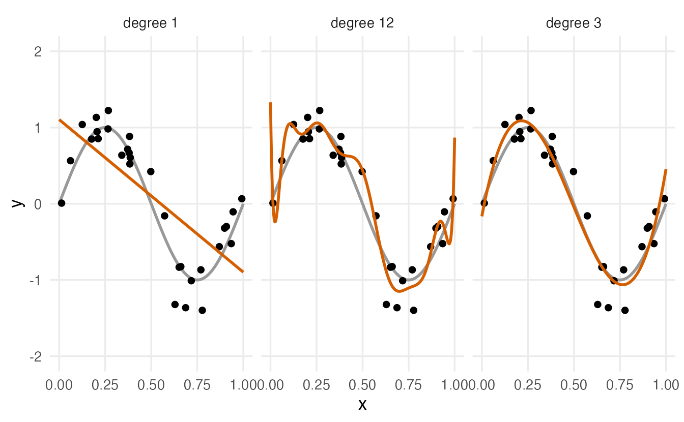

Figure 2: Fits of degree 1 (underfit), 3 (about right) and 12 (overfit) to the same 30 points; grey: true curve.

6. Train/test split

In real life we do not have 1000 fresh test points. The simplest substitute is to set aside part of the data: fit on the training part, measure the error on the held-out test part.

set.seed(5)
idx <- sample(nrow(mtcars), size = 24)   # 75% for training
cars_train <- mtcars[idx, ]
cars_test  <- mtcars[-idx, ]

fit <- lm(mpg ~ wt + hp, data = cars_train)
rmse(cars_test$mpg, predict(fit, newdata = cars_test))

#> [1] 2.612

This is honest, but with small data it is noisy: the answer depends heavily on which 8 cars happened to land in the test set. Repeating the split 10 times with different seeds:

set.seed(5)
replicate(10, {
  idx <- sample(nrow(mtcars), size = 24)
  fit <- lm(mpg ~ wt + hp, data = mtcars[idx, ])
  rmse(mtcars$mpg[-idx], predict(fit, newdata = mtcars[-idx, ]))
}) |>
  round(2)

#>  [1] 2.61 1.85 3.08 2.63 3.75 2.16 1.61 2.76 2.22 2.00

The estimates range widely. Cross-validation uses the data more efficiently.

7. k-fold cross-validation, by hand

k-fold cross-validation (CV) splits the data at random into \(k\) groups (“folds”) of similar size. Each fold takes a turn as the test set while the model is fitted on the other \(k - 1\) folds. The CV estimate is the average of the \(k\) test errors. Every observation is used for testing exactly once.

cv_rmse <- function(formula, data, k = 5) {
  folds <- sample(rep(1:k, length.out = nrow(data)))   # random fold labels
  y_name <- all.vars(formula)[1]
  fold_rmse <- numeric(k)
  for (i in 1:k) {
    fit <- lm(formula, data = data[folds != i, ])      # fit on k - 1 folds
    hold_out <- data[folds == i, ]                     # test on fold i
    fold_rmse[i] <- rmse(hold_out[[y_name]], predict(fit, hold_out))
  }
  mean(fold_rmse)
}

Because the fold assignment is random, a single CV run is still somewhat noisy. Repeated CV averages several runs with different fold assignments. Let us compare five candidate models for mpg:

candidates <- list(
  "wt"                  = mpg ~ wt,
  "wt + hp"             = mpg ~ wt + hp,
  "wt + hp + qsec + drat" = mpg ~ wt + hp + qsec + drat,
  "wt + qsec + am"      = mpg ~ wt + qsec + am,
  "all 10"              = mpg ~ .
)

set.seed(4)
cv_results <- sapply(candidates, \(f) mean(replicate(20, cv_rmse(f, mtcars))))
sort(round(cv_results, 2))

#>        wt + qsec + am wt + hp + qsec + drat               wt + hp 
#>                  2.69                  2.70                  2.74 
#>                    wt                all 10 
#>                  3.17                  3.77

The model with all 10 predictors has the worst CV error (3.77 mpg), even though it has the best fit to the training data (R² = 0.87). The small models predict new cars about equally well.

WarningCross-validate the procedure, not the result

The model wt + qsec + am was found by step() on all the data. Its CV error above is optimistic, because the test folds helped choose it. An honest estimate repeats the selection inside each fold:

set.seed(6)
folds <- sample(rep(1:5, length.out = nrow(mtcars)))
honest <- sapply(1:5, \(i) {
  sel <- step(lm(mpg ~ ., data = mtcars[folds != i, ]), trace = 0)
  rmse(mtcars$mpg[folds == i], predict(sel, mtcars[folds == i, ]))
})
mean(honest)

#> [1] 2.965

The honest error of “stepwise selection” as a procedure is about 3 mpg — worse than its optimistic value. Any data-driven choice (selecting variables, tuning, transformations chosen by looking at the data) must happen inside the resampling loop. This is the core idea behind pipelines in The machine learning workflow.

Choosing complexity by CV

Back to the polynomial example: we use only the 30 training points (pretending we do not have the 1000 test points) and pick the degree by repeated 5-fold CV.

set.seed(2)
cv_degree <- sapply(1:8, \(d) {
  f <- as.formula(paste0("y ~ poly(x, ", d, ")"))
  median(replicate(20, cv_rmse(f, train)))
})
round(cv_degree, 3)

#> [1] 0.599 0.663 0.256 0.282 0.290 0.283 0.339 0.400

which.min(cv_degree)

#> [1] 3

CV picks degree 3, close to the degree with the lowest true test error in Section 5 (5). We used the median over repeats because a few folds produce huge errors at high degrees: high-degree polynomials explode near the edges of the data when a fold leaves out the extreme points.

A common refinement is the one-standard-error rule: among the models whose CV error is within one standard error of the best, pick the simplest. It guards against choosing a complex model on the basis of a difference that is just noise. You will see it again with lambda.1se in Penalized regression.

NoteGoing deeper: the same thing with rsample

Writing CV by hand shows exactly what happens. In practice, the rsample package (part of tidymodels) creates the folds and keeps track of them:

folds <- rsample::vfold_cv(mtcars, v = 5, repeats = 20)
split_1 <- folds$splits[[1]]
rsample::analysis(split_1)    # the training part of the first resample
rsample::assessment(split_1)  # the held-out part

vfold_cv(..., strata = y) stratifies the folds, which is important for imbalanced classification. From lesson 44 on, tune and workflows run the whole loop (including preprocessing) for you.

How many folds? \(k = 5\) or \(k = 10\) are standard. Larger \(k\) means each training set is closer to the full data (less pessimistic) but the estimate is more variable and more expensive. Leave-one-out CV (\(k = n\)) is a special case; for linear models it can be computed without refitting.

WarningCommon pitfalls

1. Reporting p-values of a stepwise-selected model as if the model had been fixed in advance. They are too small, and the effects too large.
2. Judging a predictive model by its training error or R². More complexity always improves them.
3. Using the test set more than once. If you look at the test error, change the model and look again, the test set has become part of training. Choose with CV on the training data; touch the test set once, at the end.
4. Selecting variables (or tuning, or scaling) on all the data before CV. Information leaks from the test folds into the model, and the CV error is optimistic.
5. Comparing AIC across models fitted to different rows (e.g. one model drops more NAs) or to different responses (y vs log(y)). The values are not comparable.

8. Check your understanding

NoteQ1. Can you use an F-test to compare y ~ a + b with y ~ a + c?

No: neither model is a special case of the other. Use AIC/BIC or cross-validation.

NoteQ2. AIC prefers model A by 0.8 points over model B, which has two fewer predictors. Which would you choose?

A difference below 2 is negligible; most analysts would choose the simpler model B (same logic as the one-standard-error rule).

NoteQ3. Why does the training error keep decreasing as complexity grows, while the test error eventually increases?

Extra flexibility always lets the model follow the training points more closely — including their random noise. That noise does not repeat in new data, so the fitted wiggles become errors.

9. Exercises

★ Exercise 1 — F-test. Using penguins, test whether adding sex to body_mass ~ flipper_len + species improves the model. Careful: both models must be fitted to the same rows.

TipSolution

peng <- penguins |> drop_na(body_mass, flipper_len, species, sex)
m_a <- lm(body_mass ~ flipper_len + species, data = peng)
m_b <- lm(body_mass ~ flipper_len + species + sex, data = peng)
anova(m_a, m_b)

Yes: F is very large (about 200) and p < 0.001. Without drop_na(), the two models would use 342 and 333 rows and anova() would stop with an error (“models were not all fitted to the same size of dataset”).

★★ Exercise 2 — AIC by hand. For m2 <- lm(mpg ~ wt + hp, data = mtcars), compute AIC from logLik(m2) and check it against AIC(m2). How many parameters does R count?

TipSolution

ll <- logLik(m2)
attr(ll, "df")                   # 4: intercept, wt, hp and sigma
-2 * as.numeric(ll) + 2 * attr(ll, "df")
AIC(m2)

Both give about 156.7. The residual standard deviation \(\sigma\) counts as a parameter.

★★ Exercise 3 — predict the output. In the noise simulation, what would you expect the cross-validated RMSE of the stepwise-selected model to be, compared with simply predicting the mean of y for everyone? Check by computing the honest CV error (selection inside the folds) for noise and for the intercept-only model y ~ 1. (It takes a few seconds.)

TipSolution

set.seed(10)
folds <- sample(rep(1:5, length.out = nrow(noise)))
cv_step <- sapply(1:5, \(i) {
  sel <- step(lm(y ~ ., data = noise[folds != i, ]), trace = 0)
  rmse(noise$y[folds == i], predict(sel, noise[folds == i, ]))
})
cv_null <- sapply(1:5, \(i) {
  rmse(noise$y[folds == i], mean(noise$y[folds != i]))
})
c(step = mean(cv_step), mean_only = mean(cv_null))

The stepwise model predicts new data worse than the plain mean (roughly 1.2 vs 1.0 for these data): its “significant” predictors are noise, and fitting them adds error. Cross-validation exposes what the p-values hid.

★★ Exercise 4 — debug. This attempt at 5-fold CV always returns 0. Find the bug.

folds <- rep(1:5, length.out = nrow(mtcars))
err <- numeric(5)
for (i in 1:5) {
  fit <- lm(mpg ~ wt, data = mtcars)
  err[i] <- rmse(mtcars$mpg[folds == i],
                 predict(fit, mtcars[folds == i, ])) - rmse(
                   mtcars$mpg[folds == i], fitted(fit)[folds == i])
}
mean(err)

TipSolution

The model is fitted on all of mtcars (data = mtcars) in every iteration, so the “test” fold was part of the training data and predictions equal the fitted values: the difference is always 0. Fit on mtcars[folds != i, ] and drop the second term. Also, folds should be shuffled (sample(rep(...))): mtcars is not in random order, so consecutive blocks are not random folds.

★★★ Exercise 5 — mini-analysis. Using penguins (complete cases), use repeated 5-fold CV with cv_rmse() to compare four models for body_mass: flipper_len; flipper_len + species; flipper_len + species + sex; flipper_len * species * sex. Which would you choose, and why?

TipSolution

peng <- penguins |> drop_na(body_mass, flipper_len, species, sex)
cands <- list(
  a = body_mass ~ flipper_len,
  b = body_mass ~ flipper_len + species,
  c = body_mass ~ flipper_len + species + sex,
  d = body_mass ~ flipper_len * species * sex
)
set.seed(7)
sapply(cands, \(f) mean(replicate(10, cv_rmse(f, peng))))

CV RMSE drops from about 390 g (a) to about 375 g (b) and about 295 g (c); the full three-way interaction model (d) is about the same as (c) or very slightly better. By the one-standard-error logic, (c) is a sensible choice: much simpler, nearly the same predictive accuracy.

Summary

Tool	Use it for	Code
F-test	nested linear models, same rows	anova(m_small, m_big)
AIC / BIC	any models, same response and rows (lower = better)	AIC(m1, m2), BIC(m1, m2)
Stepwise	quick exploration only — never for inference	step(m, trace = 0)
Train/test split	an honest but noisy estimate of prediction error	sample(), then predict()
k-fold CV	a more stable estimate; choosing among models	cv_rmse() above, rsample::vfold_cv()

• Decide first whether you want to explain or predict.
• Training error is optimistic; only data not used to build the model tell you how it will perform.
• p-values after data-driven selection are not valid: selection on noise produces “significant” results.
• Every data-driven step must be inside the cross-validation loop.
• Prefer the simplest model whose CV error is close to the best.

NoteFurther reading

• James, Witten, Hastie & Tibshirani, An Introduction to Statistical Learning (2e), chapters 5 (resampling) and 6 (model selection), https://www.statlearning.com
• Kuhn & Silge, Tidy Modeling with R, chapter 10 on resampling, https://www.tmwr.org
• Harrell, Regression Modeling Strategies, chapter 4 — on the problems of stepwise selection, https://hbiostat.org/rmsc/