library(dplyr)
library(ggplot2)Proportions and chi-square tests
Inference for categorical data: one and two proportions, goodness of fit, independence
Test and estimate proportions with binom.test() and prop.test(), compute risk differences, relative risks and odds ratios, and analyse contingency tables with chi-square and Fisher tests, residuals and Cramér’s V.
NoteLearning objectives
By the end of this lesson you will be able to:
- test and estimate one proportion with
binom.test()andprop.test(); - compare two proportions and report the difference, the relative risk and the odds ratio;
- run a chi-square goodness-of-fit test and a chi-square test of independence;
- use expected counts, standardized residuals and Cramér’s V to describe an association;
- choose Fisher’s exact test when counts are small, and McNemar’s test for paired proportions.
1. Why special tests for categories?
Many questions are about counts, not measurements: Did a passenger survive? Which island does a penguin live on? Was a student admitted? There is no mean to compare; instead we compare proportions, or ask whether two categorical variables are associated. The logic is the one of Hypothesis testing — a null model, a test statistic, a p-value, a confidence interval — but the statistics are built from counts.
| Question | Test | R |
|---|---|---|
| Is one proportion equal to a reference value? | Exact binomial / one-sample proportion test | binom.test(x, n, p), prop.test(x, n, p) |
| Do two groups have the same proportion? | Two-sample proportion test | prop.test(table_2x2) |
| Do counts follow given proportions? | Chi-square goodness of fit | chisq.test(x, p = ...) |
| Are two categorical variables associated? | Chi-square test of independence | chisq.test(table) |
| Same, with small expected counts | Fisher’s exact test | fisher.test(table) |
| Paired yes/no outcomes (before/after) | McNemar’s test | mcnemar.test(table) |
2. One proportion
A drug leaflet states that 20% of patients experience a side effect. In a clinic, 16 of 50 patients report it. Is that compatible with 20%?
side <- binom.test(x = 16, n = 50, p = 0.20)
side
#>
#> Exact binomial test
#>
#> data: 16 and 50
#> number of successes = 16, number of trials = 50, p-value = 0.05
#> alternative hypothesis: true probability of success is not equal to 0.2
#> 95 percent confidence interval:
#> 0.1952 0.4670
#> sample estimates:
#> probability of success
#> 0.32
TipHow to read this output
- number of successes / trials: 16 of 50, so \(\hat p =\) 0.32.
- p-value: 0.049. If the true rate were 20%, a count at least as far from the expected 10 as 16 would occur with this probability. The test is exact: it uses the binomial distribution directly, no approximation.
- 95% CI: 0.195 to 0.467 — the rates compatible with the data (see Confidence intervals). It only just includes 0.20, even though the p-value is just below 0.05: the exact interval and the exact p-value are computed in slightly different ways, so at the boundary they can disagree.
prop.test() gives an approximate version based on the normal distribution (with a continuity correction):
prop.test(16, 50, p = 0.20)$p.value#> [1] 0.05183Here the two p-values fall on opposite sides of 0.05 (0.049 versus 0.052). This is a good reminder from Hypothesis testing: the evidence is borderline either way, and 0.05 is not a magic line. For a single proportion with modest \(n\), prefer the exact binom.test().
3. Two proportions: the Titanic
The built-in Titanic table cross-classifies the 2,201 people on board by class, sex, age and survival. Let us collapse it to sex × survival with margin.table() (equivalent to apply(Titanic, c(2, 4), sum)):
sex_surv <- margin.table(Titanic, c(2, 4))[, c("Yes", "No")]
sex_surv
#> Survived
#> Sex Yes No
#> Male 367 1364
#> Female 344 126prop.table(sex_surv, margin = 1) # proportions within each row#> Survived
#> Sex Yes No
#> Male 0.2120 0.7880
#> Female 0.7319 0.2681We put “Yes” first because prop.test() treats the first column as “success”. Then:
two <- prop.test(sex_surv)
two
#>
#> 2-sample test for equality of proportions with continuity correction
#>
#> data: sex_surv
#> X-squared = 454, df = 1, p-value <2e-16
#> alternative hypothesis: two.sided
#> 95 percent confidence interval:
#> -0.5657 -0.4741
#> sample estimates:
#> prop 1 prop 2
#> 0.2120 0.7319
TipHow to read this output
- prop 1, prop 2: survival proportions for the first row (Male, 0.212) and the second row (Female, 0.732).
- 95% CI: for prop 1 − prop 2, i.e. male − female: from -0.566 to -0.474. Women’s survival probability was roughly 47 to 57 percentage points higher.
- X-squared and p-value: the test of “equal proportions”. The p-value is essentially zero.
Three ways to describe the difference
The risk difference is what prop.test() reports. Two other measures are common, especially in medicine and epidemiology:
p_male   <- sex_surv["Male", "Yes"]   / sum(sex_surv["Male", ])
p_female <- sex_surv["Female", "Yes"] / sum(sex_surv["Female", ])

risk_diff <- p_female - p_male
rel_risk  <- p_female / p_male

odds_female <- sex_surv["Female", "Yes"] / sex_surv["Female", "No"]
odds_male   <- sex_surv["Male", "Yes"]   / sex_surv["Male", "No"]
odds_ratio  <- odds_female / odds_male

c(risk_diff = risk_diff, rel_risk = rel_risk, odds_ratio = odds_ratio)
#> risk_diff rel_risk odds_ratio
#> 0.5199 3.4522 10.1470- Risk difference (0.52): women’s survival probability was 52 percentage points higher.
- Relative risk (3.45): women were 3.5 times as likely to survive as men.
- Odds ratio (10.1): the odds of survival (survivors per non-survivor) were about 10 times higher for women. Odds ratios are always further from 1 than relative risks when the outcome is common, so do not read an odds ratio of 10 as “10 times as likely”. Odds ratios return in Logistic regression.
NoteGoing deeper: a CI for the odds ratio
For a 2×2 table with cells \(a, b, c, d\), \(\log(\text{OR})\) is approximately normal with standard error \(\sqrt{1/a + 1/b + 1/c + 1/d}\):
se_log_or <- sqrt(sum(1 / sex_surv))
exp(log(odds_ratio) + c(-1, 1) * qnorm(0.975) * se_log_or)
#> [1] 8.027 12.827fisher.test(sex_surv) also reports an odds ratio with a CI (a slightly different, “conditional” estimate). Careful: it compares the first row with the second, so it gives about 0.1 (male versus female), the reciprocal of ours.
4. Chi-square goodness of fit
Do observed counts match proportions fixed in advance? Gregor Mendel’s classic pea experiment produced 556 seeds in four categories; his theory predicted the ratio 9 : 3 : 3 : 1.
peas <- c(round_yellow = 315, round_green = 108,
          wrinkled_yellow = 101, wrinkled_green = 32)
gof <- chisq.test(peas, p = c(9, 3, 3, 1) / 16)
gof
#>
#> Chi-squared test for given probabilities
#>
#> data: peas
#> X-squared = 0.47, df = 3, p-value = 0.9gof$expected#> round_yellow round_green wrinkled_yellow wrinkled_green
#> 312.75 104.25 104.25 34.75The statistic compares each observed count \(O\) with its expected count \(E\) under \(H_0\):
\[ X^2 = \sum \frac{(O - E)^2}{E}. \]
If the theory is right, \(X^2\) is small. Here \(X^2 =\) 0.47 and \(p =\) 0.93: the counts are very close to what the 9:3:3:1 theory predicts. (A large p-value does not prove the theory; it says the data give no reason to doubt it.)
A second example: are the three penguin species equally represented in the data?
chisq.test(table(penguins$species)) # default p: all categories equal#>
#> Chi-squared test for given probabilities
#>
#> data: table(penguins$species)
#> X-squared = 32, df = 2, p-value = 1e-07No: Chinstrap penguins are clearly under-represented. This tells us about the sampling of the study, not necessarily about the species’ populations.
5. Chi-square test of independence
Now two variables: was survival associated with class on the Titanic?
as.data.frame(Titanic) |>
  summarise(n = sum(Freq), .by = c(Class, Survived)) |>
  ggplot(aes(Class, n, fill = Survived)) +
  geom_col(position = "fill") +
  labs(x = NULL, y = "Proportion within class", fill = "Survived")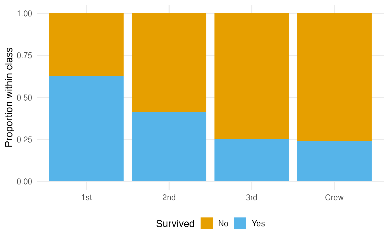
class_surv <- margin.table(Titanic, c(1, 4))
class_surv
#> Survived
#> Class No Yes
#> 1st 122 203
#> 2nd 167 118
#> 3rd 528 178
#> Crew 673 212chi <- chisq.test(class_surv)
chi#>
#> Pearson's Chi-squared test
#>
#> data: class_surv
#> X-squared = 190, df = 3, p-value <2e-16\(H_0\) is independence: the survival probability is the same in every class. Under \(H_0\), the expected count in each cell is
\[ E = \frac{\text{row total} \times \text{column total}}{\text{grand total}} . \]
round(chi$expected, 1)#> Survived
#> Class No Yes
#> 1st 220.0 105.0
#> 2nd 192.9 92.1
#> 3rd 477.9 228.1
#> Crew 599.1 285.9The test compares the observed table with this “independence table”. With \(X^2 =\) 190.4 on 3 degrees of freedom (\((\text{rows} - 1) \times (\text{columns} - 1)\)), the p-value is tiny: survival and class are associated.
Where is the association? Standardized residuals
A significant chi-square says that the table departs from independence, not where. The standardized residuals answer this. Each is roughly a z-score: values beyond about ±2 flag cells with clearly more (positive) or fewer (negative) people than independence predicts.
round(chi$stdres, 1)#> Survived
#> Class No Yes
#> 1st -12.6 12.6
#> 2nd -3.5 3.5
#> 3rd 4.9 -4.9
#> Crew 6.9 -6.9
TipHow to read the residuals
- 1st class, Yes: 12.6 — far more first-class survivors than independence would predict.
- 3rd class and Crew, No: positive residuals (4.9 and 6.9) — more deaths than expected.
- The residuals tell the story behind the single p-value: survival chances fell from first class to third class and crew.
How strong is the association? Cramér’s V
Like any p-value, the chi-square p-value depends on the sample size. Cramér’s V is an effect size between 0 (independence) and 1 (perfect association):
\[ V = \sqrt{\frac{X^2}{n\,(k - 1)}}, \qquad k = \min(\text{rows}, \text{columns}). \]
cramers_v <- function(tab) {
  x2 <- suppressWarnings(chisq.test(tab, correct = FALSE))$statistic
  k  <- min(dim(tab))
  unname(sqrt(x2 / (sum(tab) * (k - 1))))
}
cramers_v(class_surv)
#> [1] 0.2941cramers_v(sex_surv)#> [1] 0.4556The association of survival with sex (V = 0.46) is stronger than with class (V = 0.29). As a very rough guide, V around 0.1 is weak, 0.3 moderate and 0.5 or more strong (for 2×2 tables; the thresholds shrink as tables get larger). correct = FALSE switches off Yates’ continuity correction, which is applied by default to 2×2 tables and would distort V.
Hair and eye colour
HairEyeColor is a 3-way table (hair × eye × sex). We collapse over sex:
hair_eye <- margin.table(HairEyeColor, c(1, 2))
hair_eye
#> Eye
#> Hair Brown Blue Hazel Green
#> Black 68 20 15 5
#> Brown 119 84 54 29
#> Red 26 17 14 14
#> Blond 7 94 10 16he_chi <- chisq.test(hair_eye)
round(he_chi$stdres, 1)#> Eye
#> Hair Brown Blue Hazel Green
#> Black 6.1 -4.3 -0.6 -2.3
#> Brown 2.2 -3.4 2.1 -0.5
#> Red -0.1 -2.3 1.0 2.6
#> Blond -8.3 10.0 -2.7 0.7The p-value is <2e-16, and the residuals locate the association: blond hair with blue eyes (10) and black hair with brown eyes (6.1) occur much more often than independence predicts, while blond hair with brown eyes is rare (-8.3). Cramér’s V is 0.28.
A warning from Berkeley: UCBAdmissions
In 1973, the graduate school of UC Berkeley admitted men at a higher rate than women:
ucb <- margin.table(UCBAdmissions, c(2, 1))   # Gender x Admit
prop.table(ucb, margin = 1)
#> Admit
#> Gender Admitted Rejected
#> Male 0.4452 0.5548
#> Female 0.3035 0.6965The difference is very significant (chisq.test(ucb) gives \(p \approx\) 10^{-21}). But look department by department:
round(apply(UCBAdmissions, 3, \(t) t["Admitted", ] / colSums(t)), 2)#> Dept
#> Admit A B C D E F
#> Male 0.62 0.63 0.37 0.33 0.28 0.06
#> Female 0.82 0.68 0.34 0.35 0.24 0.07In most departments the admission rates of men and women are similar, and in department A women do better. The overall gap appears because women applied more often to departments that admitted few applicants of either sex. This reversal is called Simpson’s paradox: an association in a collapsed table can disappear or reverse within subgroups. A chi-square test answers the question you ask it — choose the table carefully.
Penguins: species × island
sp_isl <- table(penguins$species, penguins$island)
sp_isl
#>
#> Biscoe Dream Torgersen
#> Adelie 44 56 52
#> Chinstrap 0 68 0
#> Gentoo 124 0 0si_chi <- suppressWarnings(chisq.test(sp_isl))
round(si_chi$expected, 1)#>
#> Biscoe Dream Torgersen
#> Adelie 74.2 54.8 23.0
#> Chinstrap 33.2 24.5 10.3
#> Gentoo 60.6 44.7 18.7The association is overwhelming (Cramér’s V = 0.66): Gentoo penguins live only on Biscoe and Chinstraps only on Dream. Two lessons here. First, the table contains structural zeros — a test of “independence” is hardly informative when the answer is obvious from the table. Second, R warns that the approximation “may be incorrect” because some expected counts are small (Chinstrap on Torgersen: 10.3), which brings us to the next section.
6. Small expected counts: Fisher’s exact test
The chi-square p-value relies on an approximation that works well when all expected counts are at least about 5. When some are smaller, use Fisher’s exact test, which computes the p-value directly from the possible tables with the same margins.
Consider only the 109 children on the Titanic, in the three passenger classes:
children <- Titanic[1:3, , "Child", ] |> margin.table(c(1, 3))
children
#> Survived
#> Class No Yes
#> 1st 0 6
#> 2nd 0 24
#> 3rd 52 27suppressWarnings(chisq.test(children))$expected#> Survived
#> Class No Yes
#> 1st 2.862 3.138
#> 2nd 11.450 12.550
#> 3rd 37.688 41.312fisher.test(children)#>
#> Fisher's Exact Test for Count Data
#>
#> data: children
#> p-value = 3e-11
#> alternative hypothesis: two.sidedSome expected counts are below 5 (first class), so chisq.test() would warn. Fisher’s test is exact and gives \(p =\) 3e-11: all first- and second-class children survived, compared with about a third of the third-class children. Fisher’s test works for any table size, though it can become slow for large tables with many counts (for the penguins table above it fails with a workspace error; chisq.test(tab, simulate.p.value = TRUE) is an alternative).
7. Paired proportions: McNemar’s test
If the same people answer a yes/no question twice (before/after, two raters, two diagnostic tests), the two proportions are not independent and prop.test() is wrong — this is the categorical version of the paired t-test. A classic example (from ?mcnemar.test): 1,600 people were asked twice, a month apart, whether they approved of the US President.
approval <- matrix(c(794, 86, 150, 570), nrow = 2,
                   dimnames = list(first  = c("Approve", "Disapprove"),
                                   second = c("Approve", "Disapprove")))
approval
#> second
#> first Approve Disapprove
#> Approve 794 150
#> Disapprove 86 570mcnemar.test(approval)#>
#> McNemar's Chi-squared test with continuity correction
#>
#> data: approval
#> McNemar's chi-squared = 17, df = 1, p-value = 4e-05Only the discordant cells matter: 150 people switched from approve to disapprove, 86 the other way. McNemar’s test asks whether these two numbers differ more than chance would allow — here they do: approval fell.
WarningCommon pitfalls
- Running
chisq.test()on proportions or percentages instead of raw counts. The test needs counts; the sample size matters. - Ignoring small expected counts. Check
$expected; if several are below 5, usefisher.test()(or a simulated p-value). - Stopping at the p-value. Look at the standardized residuals to see where the association is, and report an effect size (risk difference, relative risk, odds ratio, Cramér’s V).
- Using
prop.test()for paired data. Before/after on the same people needsmcnemar.test(). - Collapsing tables carelessly. A pooled table can hide or reverse the association within subgroups (Simpson’s paradox).
- Reading an odds ratio as a relative risk. They are close only when the outcome is rare.
8. Check your understanding
9. Exercises
Interactive (run in your browser)
★ Exercise 1 — one proportion. Among the Gentoo penguins whose sex is recorded, is the proportion of females different from 0.5? Fill in the counts and run an exact test.
binom.test(successes, trials, p = reference).
binom.test(n_female, n_known, p = 0.5)There are 58 females out of 119; the p-value is large (about 0.85) and the 95% CI (about 0.39 to 0.58) contains 0.5. The data are compatible with a balanced sex ratio.
★★ Exercise 2 — chi-square or Fisher? In mtcars, is the transmission (am) associated with the number of cylinders (cyl)? Build the table, inspect the expected counts, and choose the appropriate test.
The expected counts are in $expected. If some are below 5, use fisher.test().
tab <- table(mtcars$am, mtcars$cyl)
chisq.test(tab)$expected   # R also warns: several counts below 5
fisher.test(tab)           # p about 0.009
Three of the six expected counts are below 5, so the chi-square approximation is doubtful and R warns. Fisher’s exact test gives \(p \approx 0.009\): manual cars tend to have fewer cylinders (most 8-cylinder cars are automatic).
★★★ Exercise 3 — residuals and Cramér’s V. Use only the female slice of HairEyeColor (HairEyeColor[, , "Female"]). Run the chi-square test, find the cell with the largest positive standardized residual, and compute Cramér’s V with the function from Section 5.
Standardized residuals are in $stdres. Pass the table female to cramers_v().
round(res$stdres, 1)
cramers_v(female)
The largest positive residual is again blond hair / blue eyes. Cramér’s V (about 0.3) indicates a moderate association, similar to the one for both sexes combined. R warns because one expected count (red hair, green eyes) is below 5; with p-values this small the conclusion is not in doubt, but fisher.test(female, simulate.p.value = TRUE) would confirm it.
Practice on your own computer
★★ Exercise 4 — Simpson’s paradox in detail. For each of the six departments in UCBAdmissions, run prop.test() comparing the admission rates of men and women, and collect the p-values. In which department is the difference significant, and in which direction?
TipSolution
p_dept <- sapply(dimnames(UCBAdmissions)$Dept, \(d) {
  tab <- t(UCBAdmissions[, , d])   # rows = Gender, columns = Admitted/Rejected
  prop.test(tab)$p.value
})
round(p_dept, 4)
round(apply(UCBAdmissions, 3, \(t) t["Admitted", ] / colSums(t)), 2)
Only department A shows a clear difference (p ≈ 0.0001), and it favours women (about 82% admitted versus 62% of men). In the other departments the differences are small and non-significant. The overall advantage for men comes from the different choice of departments, not from bias within departments.
★★ Exercise 5 — interpret. A study reports: “Smokers had higher odds of the disease (OR = 2.5, 95% CI 1.1 to 5.7, p = 0.03, n = 180).” A newspaper writes “Smoking makes the disease 2.5 times more likely.” Give two reasons why this sentence may be wrong.
TipSolution
- An odds ratio is not a relative risk: if the disease is common, the relative risk is closer to 1 than 2.5. (2) The study is observational and “makes … more likely” implies causation; an association can be due to confounding. One could add: the CI is wide (1.1 to 5.7), so the size of the association is very uncertain.
Summary
| Task | Code | Report |
|---|---|---|
| One proportion | binom.test(x, n, p = p0) |
\(\hat p\), 95% CI, p |
| Two proportions | prop.test(tab_2x2) (first column = success) |
difference, 95% CI; RR and OR |
| Goodness of fit | chisq.test(counts, p = probs) |
\(X^2\), df, p |
| Independence | chisq.test(tab); $expected; $stdres |
\(X^2\), df, p, Cramér’s V, key residuals |
| Small expected counts | fisher.test(tab) |
p (and OR for 2×2) |
| Paired yes/no | mcnemar.test(tab_2x2) |
discordant counts, p |
- Categorical tests compare observed counts with the counts expected under \(H_0\).
- Check expected counts; switch to Fisher’s exact test when they are small.
- Standardized residuals show where the association is; Cramér’s V shows how strong.
- Risk difference, relative risk and odds ratio answer different questions — say which one you report.
- Be careful when collapsing tables: subgroups can tell a different story.