Deep neural networks for tabular data

How a network learns, how to stop it from overfitting, and whether it beats boosting

Train a regularised feed-forward neural network with keras3 on the bank-marketing data: loss, gradient descent, backpropagation, epochs and mini-batches, dropout, weight decay and early stopping, compared with logistic regression and gradient boosting.

Level 4 · Models & learning ⏱ ~90 min Prerequisites: Deep learning set-up, The ML workflow, Gradient boosting

Learning objectives

By the end of this lesson you will be able to:

explain the training loop of a network: loss, gradient descent, backpropagation, epochs and mini-batches;
prepare a mixed numeric/categorical table for keras with a recipes pipeline estimated on the training set only;
build, compile and fit a feed-forward network with keras_model_sequential(), layer_dense(), compile() and fit();
recognise overfitting in a learning curve and control it with dropout, weight decay and early stopping;
compare the network honestly with logistic regression and gradient boosting on a held-out test set.

library(dplyr)
library(readr)
library(ggplot2)
library(rsample)
library(recipes)
library(parsnip)
library(workflows)
library(yardstick)

library(keras3)

Running this lesson

The model chunks need keras3 and a backend (see lesson 61). The results on this page were computed once on the instructor’s computer and frozen. If keras is not installed, the keras code is shown but not run, and numbers that depend on it read “not computed”. Your own numbers will differ slightly from those shown here: training a network is random.

1. Why a network for a table?

A Portuguese bank phoned its customers to sell a term deposit. For each call we know the customer’s age, job, balance, previous contacts and so on, and whether they subscribed (y). The marketing team asks: who is likely to say yes? That is a binary classification problem, exactly like those of the logistic-regression and boosting lessons.

This lesson uses the problem to learn how networks are trained. It also asks an honest question: on a table of a few thousand rows, is a neural network actually better than the classical models? (Spoiler from lesson 61: often it is not, and that is a useful result.)

2. How a network learns

2.1 Loss and gradient descent

A network is a function with many parameters (weights). Training means choosing the weights that make a loss small. For a yes/no outcome the loss is the binary cross-entropy — the same log-loss that logistic regression minimises:

\[ \mathcal L = -\frac1n\sum_{i=1}^n \big[y_i\log\hat p_i + (1-y_i)\log(1-\hat p_i)\big]. \]

A confident correct prediction ($\hat p_i$ close to $y_i$) costs almost nothing; a confident wrong one costs a lot. As in lesson 61, the weights are found by gradient descent: compute the slope of the loss with respect to each weight, take a small step downhill, repeat.

2.2 Backpropagation: the chain rule, backwards

With hidden layers, how does a weight deep inside the network know how it affected the loss? Backpropagation answers this with the chain rule of calculus: the error at the output is passed backwards, layer by layer, and each layer multiplies it by its own local derivative. One forward pass computes the predictions; one backward pass computes all the gradients.

Here is a complete network trained in base R: 2 inputs, one hidden layer of 8 tanh neurons, a sigmoid output. The data are points in a square; the class is “inside a circle”, a boundary no straight line can draw.

set.seed(42)
n <- 400
x <- matrix(runif(2 * n, -1, 1), ncol = 2)
y <- as.numeric(rowSums(x^2) < 0.5)        # 1 = inside the circle

fit_lr <- glm(y ~ x, family = binomial)    # a single neuron
acc_lr <- mean((fitted(fit_lr) > 0.5) == y)

sigmoid <- function(z) 1 / (1 + exp(-z))
forward <- function(x, par) {
  h <- tanh(sweep(x %*% par$W1, 2, par$b1, "+"))   # hidden layer
  list(h = h, p = drop(sigmoid(h %*% par$W2 + par$b2)))
}

set.seed(1)
k <- 8                                             # hidden neurons
par <- list(W1 = matrix(rnorm(2 * k), 2, k), b1 = rep(0, k),
            W2 = matrix(rnorm(k, sd = 0.5), k, 1), b2 = 0)
eta <- 0.5
for (epoch in 1:3000) {
  f <- forward(x, par)                             # forward pass
  d_out <- (f$p - y) / n                           # error at the output
  d_h <- (d_out %*% t(par$W2)) * (1 - f$h^2)       # backwards through tanh
  par$W2 <- par$W2 - eta * t(f$h) %*% d_out
  par$b2 <- par$b2 - eta * sum(d_out)
  par$W1 <- par$W1 - eta * t(x) %*% d_h
  par$b1 <- par$b1 - eta * colSums(d_h)
}
acc_nn <- mean((forward(x, par)$p > 0.5) == y)

The single neuron (logistic regression) classifies 60% of the points correctly — no better than always guessing “outside”, because a straight line cannot separate a disc. The 8-neuron network reaches 100%.

grid <- expand.grid(x1 = seq(-1, 1, length.out = 120),
                    x2 = seq(-1, 1, length.out = 120))
grid$p <- forward(as.matrix(grid), par)$p
ggplot(grid, aes(x1, x2)) +
  geom_raster(aes(fill = p > 0.5), alpha = 0.35) +
  geom_point(data = data.frame(x1 = x[, 1], x2 = x[, 2], cls = factor(y)),
             aes(colour = cls), size = 1) +
  coord_equal() +
  labs(fill = "predicted inside", colour = "true class")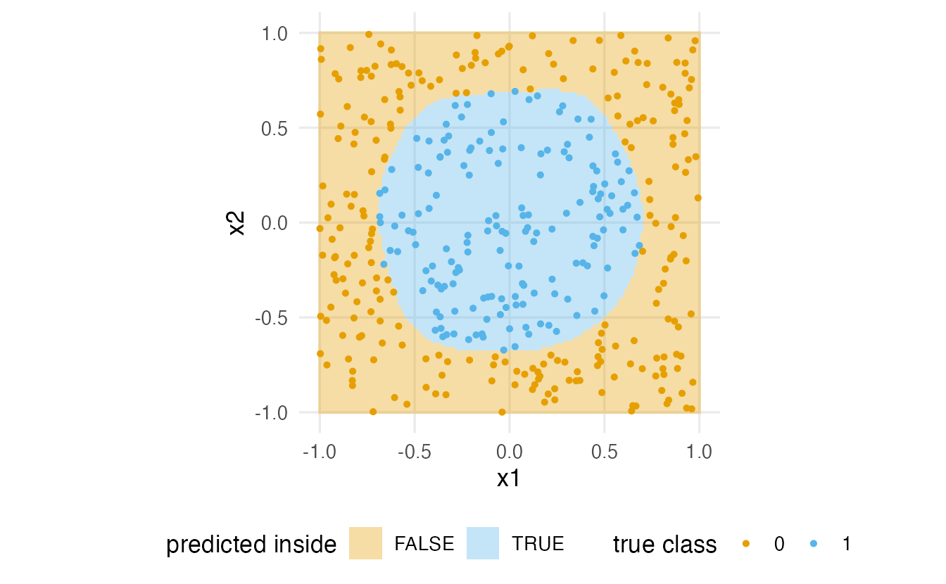

Figure 1: Decision regions of the hand-made network (shaded) and the training points. Eight tanh neurons are enough to bend the boundary into a closed curve.

Going deeper: the backpropagation formulas in the code

Write $a = XW_1 + b_1$, $h = \tanh(a)$, $\hat p = \sigma(hW_2 + b_2)$. For cross-entropy with a sigmoid output, $\partial\mathcal L/\partial(\text{output logit}) = (\hat p - y)/n$ (d_out). The chain rule gives

\[ \frac{\partial \mathcal L}{\partial W_2} = h^\top d_{\text{out}}, \qquad d_h = \big(d_{\text{out}} W_2^\top\big)\odot(1-h^2), \qquad \frac{\partial \mathcal L}{\partial W_1} = X^\top d_h, \]

where $1-h^2$ is the derivative of $\tanh$ and $\odot$ is element-wise multiplication. keras does exactly this automatically (“automatic differentiation”) for any architecture you build.

2.3 Epochs and mini-batches

Our base-R loop used all 400 points for every step. With large data that is slow, so keras uses mini-batch gradient descent: shuffle the rows, cut them into batches of, say, 64 rows, and take one step per batch. One pass through all batches is an epoch. With $n$ training rows and batch size $B$ there are $\lceil n/B\rceil$ weight updates per epoch. Small batches give noisy but frequent steps; large batches give smoother but fewer steps. The optimiser Adam, used below, is gradient descent that adapts the step size of each weight automatically.

3. The data

bank_raw <- read_delim(data_path("bank_marketing.csv"), delim = ";",
                       show_col_types = FALSE)
dim(bank_raw)

#> [1] 4521   17

count(bank_raw, y)

#> # A tibble: 2 × 2
#>   y         n
#>   <chr> <int>
#> 1 no     4000
#> 2 yes     521

The file is semicolon-separated (common in countries that use the comma as decimal mark), hence read_delim(delim = ";"). Only about 12% of customers said yes: the classes are imbalanced, so accuracy alone would be misleading (always predicting “no” is already 88% accurate). We will use the ROC AUC and the log-loss.

Two cleaning decisions, both row-by-row (so they can be done before splitting without leakage):

duration is removed. It is the length of the call, known only after the call has ended — and a customer who subscribes obviously stays on the phone longer. Using it would give an impressive but useless model (the original lesson included it; this version fixes that).
pdays = -1 means “never contacted before”, not a number of days. We add an indicator prev_contacted and set those pdays to 0.

bank <- bank_raw |>
  mutate(
    y = factor(y, levels = c("no", "yes")),
    prev_contacted = as.numeric(pdays != -1),
    pdays = if_else(pdays == -1, 0, pdays),
    across(where(is.character), as.factor)
  ) |>
  select(-duration)

4. Train, validation and test sets

A network needs a validation set while it trains (to decide when to stop and to compare settings), and we need an untouched test set for the final comparison. A stratified 70/15/15 split keeps the share of “yes” similar in the three parts.

set.seed(2024)
bank_split <- initial_validation_split(bank, prop = c(0.70, 0.15), strata = y)
bank_train <- training(bank_split)
bank_valid <- validation(bank_split)
bank_test  <- testing(bank_split)
c(train = nrow(bank_train), valid = nrow(bank_valid), test = nrow(bank_test))

#> train valid  test 
#>  3164   678   679

5. Preprocessing with a recipe

Networks need numeric inputs on comparable scales: a balance in thousands of euros and an indicator 0/1 would otherwise receive very different step sizes. The recipe turns each categorical variable into dummy columns, drops any column that is constant in the training data, and standardises everything — with means and standard deviations estimated on the training set only.

bank_rec <- recipe(y ~ ., data = bank_train) |>
  step_dummy(all_nominal_predictors()) |>
  step_zv(all_predictors()) |>
  step_normalize(all_numeric_predictors())
bank_prep <- prep(bank_rec)

to_matrix <- function(data) {
  bake(bank_prep, new_data = data, all_predictors(), composition = "matrix")
}
x_train <- to_matrix(bank_train)
x_valid <- to_matrix(bank_valid)
x_test  <- to_matrix(bank_test)
y_train <- as.numeric(bank_train$y == "yes")
y_valid <- as.numeric(bank_valid$y == "yes")
y_test  <- as.numeric(bank_test$y == "yes")
dim(x_train)

#> [1] 3164   42

After preprocessing each customer is a row of 42 numbers. (The original lesson built the dummy columns separately on each split with model.matrix(); that breaks as soon as a rare category is missing from one split. A prepped recipe always produces the same columns.)

6. Classical baselines first

Before any network, two models from earlier lessons, fitted with the same recipe on the training set and scored on the validation set.

prob_yes <- function(fit, data) predict(fit, data, type = "prob")$.pred_yes
auc <- function(p, data) roc_auc_vec(data$y, p, event_level = "second")

log_fit <- workflow(bank_rec, logistic_reg()) |>
  fit(data = bank_train)

set.seed(2024)
xgb_spec <- boost_tree(trees = 500, tree_depth = 3, learn_rate = 0.02) |>
  set_engine("xgboost") |>
  set_mode("classification")
xgb_fit <- workflow(bank_rec, xgb_spec) |>
  fit(data = bank_train)

c(logistic = auc(prob_yes(log_fit, bank_valid), bank_valid),
  boosting = auc(prob_yes(xgb_fit, bank_valid), bank_valid))

#> logistic boosting 
#>   0.7404   0.7345

These are the numbers a network has to beat. Without duration, the problem is genuinely hard: an AUC well below 1 is expected.

7. Building the network

Design choices for a first tabular network:

two hidden layers (64 and 32 neurons) with ReLU activation — enough capacity for interactions, small enough for 3164 rows;
one sigmoid output giving $P(\text{yes})$;
dropout after each hidden layer and a small weight decay ($L_2$ penalty) on the weights (explained in Section 9).

set_random_seed(123)
dnn <- keras_model_sequential(input_shape = ncol(x_train)) |>
  layer_dense(units = 64, activation = "relu",
              kernel_regularizer = regularizer_l2(1e-4)) |>
  layer_dropout(rate = 0.3) |>
  layer_dense(units = 32, activation = "relu",
              kernel_regularizer = regularizer_l2(1e-4)) |>
  layer_dropout(rate = 0.3) |>
  layer_dense(units = 1, activation = "sigmoid")

dnn |> compile(
  optimizer = optimizer_adam(learning_rate = 1e-3),
  loss = "binary_crossentropy",
  metrics = list(metric_auc(name = "auc"))
)
dnn

#> Model: "sequential"
#> ┏━━━━━━━━━━━━━━━━━━━━━━━━━━━━━━━━━━━┳━━━━━━━━━━━━━━━━━━━━━━━━━━┳━━━━━━━━━━━━━━━┓
#> ┃ Layer (type)                      ┃ Output Shape             ┃       Param # ┃
#> ┡━━━━━━━━━━━━━━━━━━━━━━━━━━━━━━━━━━━╇━━━━━━━━━━━━━━━━━━━━━━━━━━╇━━━━━━━━━━━━━━━┩
#> │ dense (Dense)                     │ (None, 64)               │         2,752 │
#> ├───────────────────────────────────┼──────────────────────────┼───────────────┤
#> │ dropout (Dropout)                 │ (None, 64)               │             0 │
#> ├───────────────────────────────────┼──────────────────────────┼───────────────┤
#> │ dense_1 (Dense)                   │ (None, 32)               │         2,080 │
#> ├───────────────────────────────────┼──────────────────────────┼───────────────┤
#> │ dropout_1 (Dropout)               │ (None, 32)               │             0 │
#> ├───────────────────────────────────┼──────────────────────────┼───────────────┤
#> │ dense_2 (Dense)                   │ (None, 1)                │            33 │
#> └───────────────────────────────────┴──────────────────────────┴───────────────┘
#>  Total params: 4,865 (19.00 KB)
#>  Trainable params: 4,865 (19.00 KB)
#>  Non-trainable params: 0 (0.00 B)

How to read this output

The first dense layer has 42 × 64 weights + 64 biases = 2752 parameters; the second 64 × 32 + 32 = 2080; the output 32 + 1 = 33.
Dropout layers have no parameters: they only switch neurons off at random during training.
compile() attaches the loss, the optimiser and the metrics. It changes dnn in place: there is no need to re-assign it.

8. Training with a validation set and early stopping

fit() runs the epochs. At the end of each epoch keras evaluates the loss on the validation data. Early stopping watches that validation loss and stops when it has not improved for patience epochs, then restores the best weights seen.

early_stop <- callback_early_stopping(monitor = "val_loss", patience = 15,
                                      restore_best_weights = TRUE)
history <- dnn |> fit(
  x = x_train, y = y_train,
  validation_data = list(x_valid, y_valid),
  epochs = 200, batch_size = 64,
  callbacks = list(early_stop),
  verbose = 0
)
n_epochs <- length(history$metrics$loss)

With 3164 training rows and batches of 64, each epoch makes 50 weight updates. Training stopped after 25 of the allowed 200 epochs.

plot_history <- function(history, title = NULL) {
  as.data.frame(history) |>
    filter(!is.na(value)) |>
    ggplot(aes(epoch, value, colour = data)) +
    geom_line(linewidth = 0.8) +
    facet_wrap(~ metric, scales = "free_y") +
    labs(x = "Epoch", y = NULL, colour = NULL, title = title)
}

plot_history(history, "Regularised network")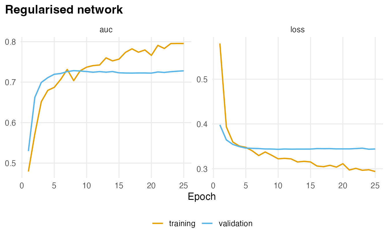

Figure 2: Learning curves of the regularised network: loss and AUC on the training and validation sets after each epoch.

How to read a learning curve

The training loss usually keeps decreasing: the network gets better and better at the data it sees.
The validation loss decreases at first and then flattens or rises. The best epoch is near its minimum; early stopping keeps the weights from that epoch.
A large, growing gap between the two curves is the signature of overfitting. With dropout active during training, the training loss can even be slightly higher than the validation loss — that is normal.

9. Overfitting and three ways to fight it

To see overfitting, train a bigger network (two layers of 256 neurons, about 77 thousand parameters) with no regularisation and no early stopping.

set_random_seed(123)
big <- keras_model_sequential(input_shape = ncol(x_train)) |>
  layer_dense(units = 256, activation = "relu") |>
  layer_dense(units = 256, activation = "relu") |>
  layer_dense(units = 1, activation = "sigmoid")
big |> compile(optimizer = optimizer_adam(learning_rate = 1e-3),
               loss = "binary_crossentropy")
history_big <- big |> fit(
  x_train, y_train, validation_data = list(x_valid, y_valid),
  epochs = 60, batch_size = 64, verbose = 0
)
best_big <- which.min(history_big$metrics$val_loss)

plot_history(history_big, "Large network, no regularisation")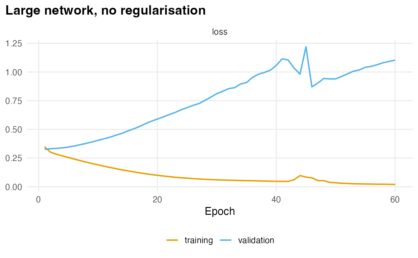

Figure 3: An unregularised network with many parameters: the training loss keeps falling while the validation loss turns upwards — overfitting.

The validation loss of the big network was lowest at epoch 1; after that, every extra epoch makes the network memorise the training customers instead of learning patterns that generalise. Three standard remedies, all used in our first model:

Remedy	What it does	keras3 code
Early stopping	Stop when validation loss stops improving; keep the best weights	`callback_early_stopping(monitor = "val_loss", patience = , restore_best_weights = TRUE)`
Weight decay ($L_2$)	Adds $\lambda\sum w^2$ to the loss: large weights are penalised, as in ridge regression	`kernel_regularizer = regularizer_l2(1e-4)`
Dropout	During training, each neuron’s output is set to 0 with probability $p$; the network cannot rely on any single neuron	`layer_dropout(rate = 0.3)`

Going deeper: dropout and weight decay

Weight decay. With penalty $\lambda\lVert W\rVert_2^2$, each gradient step becomes $w \leftarrow w - \eta(\nabla\mathcal L + 2\lambda w) = (1 - 2\eta\lambda)w - \eta\nabla\mathcal L$: the weights are shrunk (“decay”) a little at every step, exactly the shrinkage of ridge regression.

Dropout. In training, a layer’s output $h$ is replaced by $h \odot m/(1-p)$, where $m$ is a random 0/1 mask with $P(m_j = 0) = p$; dividing by $1-p$ keeps the expected value unchanged. At prediction time no units are dropped. Each mini-batch therefore trains a different “thinned” network, and the final model behaves like an average of many of them — similar in spirit to the bagging of random forests.

10. Final comparison on the test set

Only now do we touch the test set, once, for all three models.

p_test <- list(
  "Logistic regression" = prob_yes(log_fit, bank_test),
  "Gradient boosting"   = prob_yes(xgb_fit, bank_test),
  "Neural network"      = as.vector(predict(dnn, x_test, verbose = 0))
)
results <- tibble(
  model    = names(p_test),
  roc_auc  = sapply(p_test, auc, data = bank_test),
  log_loss = sapply(p_test, \(p) mn_log_loss_vec(bank_test$y, p,
                                                 event_level = "second"))
)
results

#> # A tibble: 3 × 3
#>   model               roc_auc log_loss
#>   <chr>                 <dbl>    <dbl>
#> 1 Logistic regression  0.7308   0.2926
#> 2 Gradient boosting    0.7428   0.2881
#> 3 Neural network       0.7383   0.2978

best_model <- results$model[which.max(results$roc_auc)]

How to read this output

ROC AUC (higher is better): the probability that a random “yes” customer gets a higher score than a random “no” customer. Log-loss (lower is better) also rewards well-calibrated probabilities.
In this run the highest test AUC belongs to: Gradient boosting.
The test set has only 679 customers, of whom 72 said yes. Differences of a couple of hundredths in AUC are within the noise (Exercise 5 asks you to quantify it with the bootstrap). On data like these the honest summary is usually that the network is about as good as the classical models — at a higher cost in time, tuning and interpretability.

A probability is not yet a decision. At the usual threshold of 0.5 the network’s predictions on the test set look like this:

pred_class <- factor(if_else(p_test[["Neural network"]] >= 0.5, "yes", "no"),
                     levels = c("no", "yes"))
table(truth = bank_test$y, predicted = pred_class)

#>      predicted
#> truth  no yes
#>   no  600   7
#>   yes  62  10

With rare positives, a 0.5 threshold usually catches only a minority of the “yes” customers (low recall). If calling a customer is cheap and missing a subscriber is expensive, choose a lower threshold on the validation set, exactly as in the logistic-regression lesson.

Common pitfalls

Leaking information through a predictor. duration is only known after the outcome; including it inflates every metric. Always ask “would I know this value at prediction time?”.
Scaling with the whole dataset. Means and standard deviations must come from the training set (a prepped recipe does this). Unscaled inputs also make training slow and unstable.
Judging a network by the training loss. Only validation (during development) and test (once, at the end) performance count.
Using set.seed() for keras. It does not control the weights’ initialisation or the batch shuffling; use set_random_seed().
Skipping the baseline. Without logistic regression and boosting on the same split, you cannot say whether the network was worth it.
Treating 0.5 as the only threshold with imbalanced classes.

11. Check your understanding

Q1. With 3,000 training rows and batch_size = 100, how many weight updates happen in 20 epochs?

$3000/100 = 30$ updates per epoch, so $30 \times 20 = 600$ updates.

Q2. The validation loss reaches its minimum at epoch 12 and then rises, while the training loss keeps falling. What is happening and what does early stopping with restore_best_weights = TRUE return?

The network starts overfitting after epoch 12. Early stopping halts training patience epochs later and returns the weights from epoch 12.

Q3. Why does a dropout layer have zero parameters?

It does not learn anything: it multiplies its input by a random 0/1 mask (rescaled) during training and passes it unchanged at prediction time.

Q4. Which classical method is weight decay equivalent to, in spirit?

Ridge regression: an $L_2$ penalty on the coefficients that shrinks them towards zero.

12. Exercises

★ Exercise 1 — more neurons in base R. In the base-R network of Section 2.2, change k to 2 and then to 3 hidden neurons. Can the network still draw a closed boundary? Re-plot the decision regions.

Solution

Change k <- 2 (or 3) and re-run the tiny-network and fig-circle chunks. With 2 neurons the boundary can only combine two “soft lines”, so it cannot enclose a disc and accuracy stays well below the 8-neuron network; with 3 neurons it can form a rough triangle around the circle and does much better. Capacity (number of neurons) controls how complex the boundary can be.

★★ Exercise 2 — tune the regularisation. Refit the network of Section 7 with (a) rate = 0 and no kernel_regularizer, (b) rate = 0.5 and regularizer_l2(1e-3). Keep early stopping. Compare the validation AUC (max(history$metrics$val_auc)) and the number of epochs. Remember to call set_random_seed() before each model.

Solution

fit_variant <- function(rate, l2) {
  set_random_seed(123)
  m <- keras_model_sequential(input_shape = ncol(x_train)) |>
    layer_dense(64, activation = "relu",
                kernel_regularizer = regularizer_l2(l2)) |>
    layer_dropout(rate) |>
    layer_dense(32, activation = "relu",
                kernel_regularizer = regularizer_l2(l2)) |>
    layer_dropout(rate) |>
    layer_dense(1, activation = "sigmoid")
  m |> compile(optimizer = optimizer_adam(1e-3),
               loss = "binary_crossentropy",
               metrics = list(metric_auc(name = "auc")))
  h <- m |> fit(x_train, y_train, validation_data = list(x_valid, y_valid),
                epochs = 200, batch_size = 64, verbose = 0,
                callbacks = list(callback_early_stopping(
                  monitor = "val_loss", patience = 15,
                  restore_best_weights = TRUE)))
  c(val_auc = max(h$metrics$val_auc), epochs = length(h$metrics$loss))
}
rbind(none = fit_variant(0, 0), strong = fit_variant(0.5, 1e-3))

Without regularisation the network usually stops after fewer epochs (it overfits quickly); with strong regularisation it trains longer. The validation AUCs are typically close: on this dataset the choice matters less than early stopping. Do not pick a winner from a difference in the third decimal.

★★ Exercise 3 — class weights. Refit the network adding class_weight = list("0" = 1, "1" = 5) to fit(). This makes each “yes” customer count five times in the loss. Compare the confusion matrix at threshold 0.5 with Section 10. What happens to recall? Does the AUC change much?

Solution

Add the argument to the fit() call and recompute pred_class and the table. The weighted network predicts “yes” much more often: recall for the “yes” class increases and precision decreases. The AUC, which does not depend on a threshold, changes much less: class weights mostly shift the predicted probabilities (they are no longer calibrated), which is similar to lowering the threshold.

★★ Exercise 4 — debug the pipeline. A student writes:

bank_std <- bank_raw |> mutate(across(where(is.numeric), \(v) as.numeric(scale(v))))
split <- initial_split(bank_std)

and includes duration as a predictor. Their network reaches a test AUC above 0.9. List the two problems and how to fix them.

Solution

Leakage through preprocessing: the means and standard deviations are computed on all rows, including the future test set. Fix: estimate them in a recipe prepped on the training data only. (2) Leakage through a predictor: duration is known only after the call, when the outcome is (almost) decided. Fix: remove it. The second problem is by far the bigger one and explains most of the impressive AUC. (A smaller issue: no strata = y in the split.)

★★★ Exercise 5 — is the difference real? Using the test-set probabilities in p_test, compute a 95% bootstrap confidence interval for the difference in AUC between the network and gradient boosting (resample test customers with replacement 1,000 times). Does the interval contain 0?

Solution

set.seed(1)
d <- replicate(1000, {
  i <- sample(nrow(bank_test), replace = TRUE)
  auc(p_test[["Neural network"]][i], bank_test[i, ]) -
    auc(p_test[["Gradient boosting"]][i], bank_test[i, ])
})
quantile(d, c(0.025, 0.975))

Resampling the same customers for both models (a paired bootstrap, see lesson 31) accounts for the fact that the two models are scored on identical data. With a test set of this size the interval typically contains 0: the data cannot tell the two models apart.

Summary

Step	keras3 / tidymodels code
Split with validation set	`initial_validation_split(data, prop = c(0.7, 0.15), strata = y)`
Preprocess on training only	`recipe()` with `step_dummy()`, `step_zv()`, `step_normalize()`; then `prep()` and `bake(..., composition = "matrix")`
Define the network	`keras_model_sequential(input_shape = p)`, then add `layer_dense()` and `layer_dropout()` with the pipe
Weight decay	`kernel_regularizer = regularizer_l2(1e-4)`
Loss, optimiser, metrics	`compile(optimizer = optimizer_adam(), loss = "binary_crossentropy", metrics = list(metric_auc()))`
Train	`fit(x, y, validation_data = list(xv, yv), epochs, batch_size, callbacks)`
Early stopping	`callback_early_stopping(monitor = "val_loss", patience, restore_best_weights = TRUE)`
Predict	`predict(model, x_test)`
Reproducibility	`set_random_seed(123)`

A network is trained by mini-batch gradient descent on a loss; backpropagation computes all gradients with the chain rule.
The learning curve on a validation set is the main diagnostic: a growing train–validation gap means overfitting.
Dropout, weight decay and early stopping are the standard defences.
Preprocessing is estimated on the training set; predictors unavailable at prediction time must be dropped.
On small tabular data, compare with logistic regression and boosting on the same split: the network is often no better.