Sampling distributions

Every estimate is one draw from a distribution — the idea behind all of inference

Simulate thousands of samples from a known population to see sampling variability, the standard error and its 1/sqrt(n) law, the Central Limit Theorem, unbiased estimators (including the n - 1 in the variance) and the sampling distribution of a proportion.

Level 3 · Inference ⏱ ~80 min Prerequisites: Probability distributions

NoteLearning objectives

By the end of this lesson you will be able to:

• distinguish a population from a sample and a parameter from a statistic (estimate);
• simulate the sampling distribution of a statistic and describe its centre and spread;
• compute and interpret the standard error, and explain why it shrinks like \(1/\sqrt{n}\);
• state the Central Limit Theorem and show it at work for skewed and discrete populations;
• explain what an unbiased estimator is and why the sample variance divides by \(n - 1\).

library(ggplot2)

1. Why sampling distributions?

A researcher weighs 25 penguins and reports a mean of 4,150 g. A colleague catches 25 other penguins from the same colony and gets 4,260 g. Who is right?

Both. Each sample mean is a perfectly honest summary of its sample, and each differs from the true mean of the whole colony because of which birds happened to be caught. If we could repeat the study many times, the sample means would form a distribution of their own — the sampling distribution. Its spread tells us how much to trust any single study.

In real life we see only one sample. In R we can do what researchers cannot: create a population whose truth we know, draw thousands of samples from it, and watch what the estimates do. Everything in the next module — confidence intervals, hypothesis tests, p-values — is built on what we see in this lesson.

2. Population, sample, parameter, statistic

	Population	Sample
What it is	All units we want to learn about	The units we actually observe
A number describing it	Parameter (fixed, unknown)	Statistic or estimate (known, varies from sample to sample)
Mean	\(\mu\)	\(\bar x\)
Standard deviation	\(\sigma\)	\(s\)
Proportion	\(p\)	\(\hat p\) (“p-hat”)

A statistic used to guess a parameter is called an estimator; its value in a particular sample is the estimate. Greek letters for parameters and “hats” for estimates are a convention you will see everywhere.

Let us build a population we fully know: the time (in minutes) that 100,000 visitors spent on a website. Times like these are right-skewed: most visits are short, a few are very long.

set.seed(2026)
pop <- rgamma(100000, shape = 2, scale = 5)   # a skewed population
mu    <- mean(pop)                            # the true parameters
sigma <- sd(pop)
c(mu = mu, sigma = sigma)

#>     mu  sigma 
#> 10.005  7.038

ggplot(data.frame(time = pop), aes(time)) +
  geom_histogram(bins = 60, fill = "grey70", colour = "white") +
  geom_vline(xintercept = mu, linetype = "dashed", linewidth = 1) +
  labs(x = "Time on site (minutes)", y = "Number of visitors")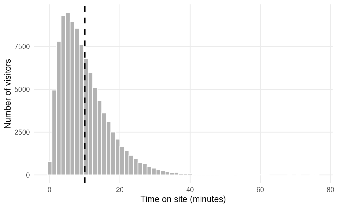

Figure 1: The simulated population of 100,000 visit times. The dashed line marks the population mean μ.

3. One sample, then many

A study observes a random sample of 25 visitors:

set.seed(1)
my_sample <- sample(pop, size = 25)
mean(my_sample)

#> [1] 8.632

The estimate 8.63 is not equal to \(\mu =\) 10. Five more studies give five more answers:

set.seed(2)
replicate(5, mean(sample(pop, size = 25)))

#> [1] 11.000  9.958  9.696  7.291 10.541

This is sampling variability: estimates change from sample to sample even though the population, the method and the sample size are identical. Now repeat the study 10,000 times and keep every mean:

set.seed(3)
means_25 <- replicate(10000, mean(sample(pop, size = 25)))
c(mean_of_means = mean(means_25), sd_of_means = sd(means_25))

#> mean_of_means   sd_of_means 
#>        10.013         1.408

ggplot(data.frame(xbar = means_25), aes(xbar)) +
  geom_histogram(bins = 50, fill = "#0072B2", colour = "white") +
  geom_vline(xintercept = mu, linetype = "dashed", linewidth = 1) +
  labs(x = "Sample mean (minutes), n = 25", y = "Number of samples")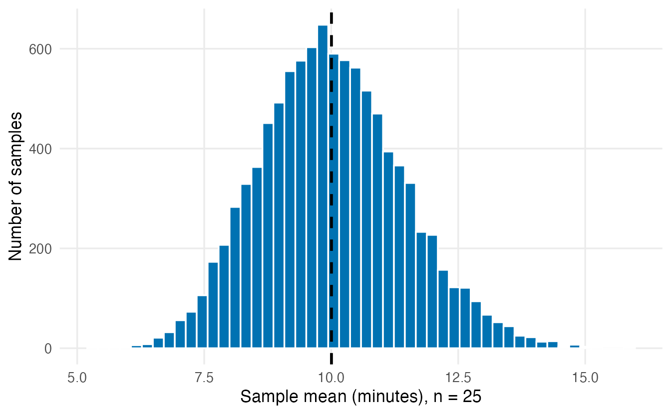

Figure 2: Sampling distribution of the mean for samples of 25 visitors (10,000 simulated studies). It is centred on μ (dashed line), much narrower than the population, and far more symmetric.

TipHow to read this plot

• Each bar counts studies, not visitors: one study = one sample mean.
• Centre: the average of the 10,000 means is 10.01, essentially \(\mu\). The sample mean does not systematically over- or under-estimate.
• Spread: a typical study misses \(\mu\) by about 1.41 minutes. That number is the standard error of the mean for \(n = 25\).
• Shape: the population is skewed, but the sample means are much closer to a bell curve. That is the Central Limit Theorem (Section 5).

4. The standard error and the \(\sqrt{n}\) law

The standard error (SE) of a statistic is the standard deviation of its sampling distribution: how far, typically, an estimate lands from the parameter. It is the single most important number for judging the precision of an estimate.

How does it depend on the sample size? Let us simulate samples of 10, 40 and 160 visitors — each four times larger than the previous one.

set.seed(4)
ns <- c(10, 40, 160)
se_df <- do.call(rbind, lapply(ns, \(n) {
  data.frame(n = n, xbar = replicate(5000, mean(sample(pop, n))))
}))
se_table <- data.frame(
  n = ns,
  simulated_se = tapply(se_df$xbar, se_df$n, sd),
  formula_se = sigma / sqrt(ns)
)
se_table

#>       n simulated_se formula_se
#> 10   10       2.2138     2.2255
#> 40   40       1.0936     1.1127
#> 160 160       0.5583     0.5564

ggplot(se_df, aes(xbar)) +
  geom_histogram(bins = 50, fill = "#009E73", colour = "white") +
  geom_vline(xintercept = mu, linetype = "dashed") +
  facet_wrap(~ n, ncol = 1, labeller = label_both) +
  labs(x = "Sample mean (minutes)", y = "Number of samples")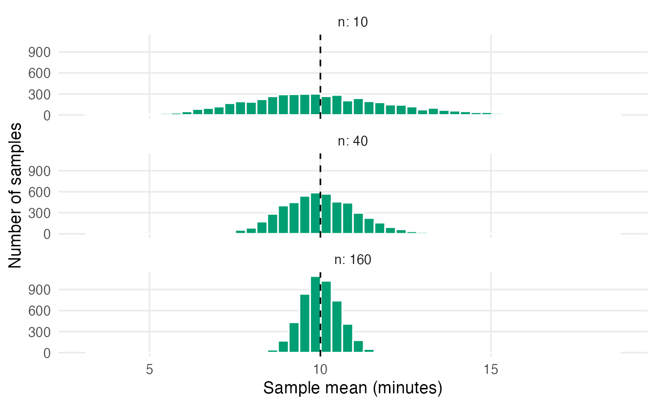

Figure 3: Sampling distributions of the mean for n = 10, 40 and 160. Each fourfold increase in n halves the spread.

The simulated SEs match the formula

\[ \operatorname{SE}(\bar x) = \frac{\sigma}{\sqrt{n}} . \]

Two consequences:

1. Bigger samples give more precise estimates, but with diminishing returns: to halve the SE you need four times as many observations.
2. The precision depends on \(n\), not on the size of the population. A sample of 1,000 is as informative about a city of 100,000 as about a country of 60 million (as long as both samples are random).

In practice \(\sigma\) is unknown, so we plug in the sample SD: the estimated standard error is \(s/\sqrt{n}\). From our single sample of 25:

sd(my_sample) / sqrt(25)   # estimated from one sample

#> [1] 1.275

sigma / sqrt(25)           # true SE (known only because we built `pop`)

#> [1] 1.408

WarningSD or SE?

The standard deviation describes the spread of the data (individual visitors). The standard error describes the spread of an estimate (sample means across studies). The SD does not shrink as you collect more data; the SE does.

NoteGoing deeper: why \(\sigma / \sqrt{n}\)?

If \(X_1, \ldots, X_n\) are independent with variance \(\sigma^2\), the variance of their sum is the sum of the variances, \(n\sigma^2\). Dividing the sum by \(n\) divides the variance by \(n^2\):

\[ \operatorname{Var}(\bar X) = \frac{n \sigma^2}{n^2} = \frac{\sigma^2}{n}, \qquad \operatorname{SD}(\bar X) = \frac{\sigma}{\sqrt n}. \]

Independence is essential: if observations are correlated (repeated measurements on the same person, neighbouring days of a time series), the SE is larger than \(\sigma/\sqrt n\). (Strictly, sampling without replacement from a finite population of size \(N\) reduces the SE by a factor \(\sqrt{(N-n)/(N-1)}\), which is negligible when \(n\) is small relative to \(N\).)

5. The Central Limit Theorem

The histogram in Section 3 was already more symmetric than the population. This is no accident. The Central Limit Theorem (CLT) says:

Whatever the shape of the population (as long as its variance is finite), the sampling distribution of the mean becomes approximately normal as the sample size grows, with mean \(\mu\) and standard deviation \(\sigma/\sqrt n\).

Let us test it on two populations that are very far from normal:

• a strongly right-skewed exponential population (rexp()), and
• a discrete population taking only the values 0 to 5, mostly 0 (think “number of cups of coffee per day”).

set.seed(5)
coffee_values <- 0:5
coffee_probs  <- c(0.45, 0.25, 0.15, 0.08, 0.05, 0.02)

clt_df <- do.call(rbind, lapply(c(2, 5, 30, 100), \(n) {
  rbind(
    data.frame(population = "Exponential", n = n,
               xbar = replicate(5000, mean(rexp(n, rate = 1)))),
    data.frame(population = "Discrete (0-5)", n = n,
               xbar = replicate(5000, mean(sample(coffee_values, n,
                                replace = TRUE, prob = coffee_probs))))
  )
}))

ggplot(clt_df, aes(xbar)) +
  geom_histogram(bins = 40, fill = "#56B4E9", colour = "white") +
  facet_grid(population ~ n, scales = "free",
             labeller = labeller(n = label_both)) +
  labs(x = "Sample mean", y = "Number of samples")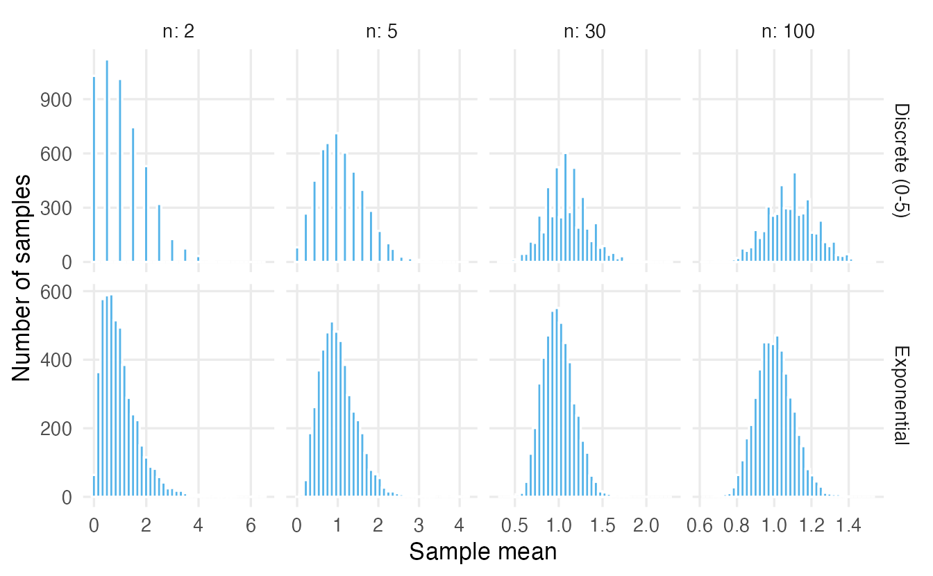

Figure 4: The Central Limit Theorem at work. Columns: sample size n. Rows: population. As n grows, the distribution of the sample mean becomes narrower and bell-shaped, whatever the population looks like.

We can also measure the asymmetry with the skewness (0 for a symmetric distribution, positive for right skew; see Summary statistics):

skew <- function(x) mean((x - mean(x))^3) / sd(x)^3
tapply(clt_df$xbar, list(clt_df$population, clt_df$n), skew)

#>                     2      5     30    100
#> Discrete (0-5) 0.8314 0.5625 0.2548 0.1309
#> Exponential    1.5493 0.9423 0.3775 0.2587

TipHow to read the CLT plots

• With n = 2 the sample means still look like the population: skewed, and for the discrete population, lumpy (only a few possible values).
• By n = 30 both are close to a bell curve, and the skewness has dropped to around 0.4 (exponential) and 0.3 (discrete).
• By n = 100 the remaining skew is small and the spread is narrow.
• “n = 30 is enough” is a rule of thumb, not a law: the more skewed the population, the larger \(n\) must be (Exercise 3 shows a population where 30 is not enough).

The CLT is why normal-based methods (t-tests, confidence intervals for means, regression) work well for averages even when the data are not normal. It does not make the data themselves normal.

NoteGoing deeper: a formal statement

Let \(X_1, X_2, \ldots\) be independent and identically distributed with mean \(\mu\) and finite variance \(\sigma^2\). Then

\[ \frac{\bar X_n - \mu}{\sigma / \sqrt n} \xrightarrow{\;d\;} N(0, 1) \quad \text{as } n \to \infty, \]

i.e. the standardised mean converges in distribution to a standard normal. The skewness of \(\bar X_n\) equals the population skewness divided by \(\sqrt n\), which is why strongly skewed populations need larger samples. The CLT also applies to sums, and hence to proportions (a proportion is the mean of 0/1 values).

6. Good estimators: unbiased and precise

An estimator is unbiased if its sampling distribution is centred on the parameter it targets: on average over many samples, it is right. A good estimator is also precise: its SE is small. Think of darts: unbiased means the darts are centred on the bullseye; precise means they are tightly grouped.

Mean versus median

For a symmetric (normal) population, the sample mean and the sample median both target the centre \(\mu\). Which is better?

set.seed(6)
est <- replicate(10000, {
  x <- rnorm(15, mean = 50, sd = 10)
  c(mean = mean(x), median = median(x))
})
rowMeans(est)          # centres: both close to 50

#>   mean median 
#>  50.00  49.97

apply(est, 1, sd)      # standard errors

#>   mean median 
#>  2.581  3.172

est_df <- data.frame(
  estimate = c(est["mean", ], est["median", ]),
  estimator = rep(c("Mean", "Median"), each = ncol(est))
)
ggplot(est_df, aes(estimate, fill = estimator)) +
  geom_density(alpha = 0.5) +
  geom_vline(xintercept = 50, linetype = "dashed") +
  labs(x = "Estimate", y = "Density", fill = NULL)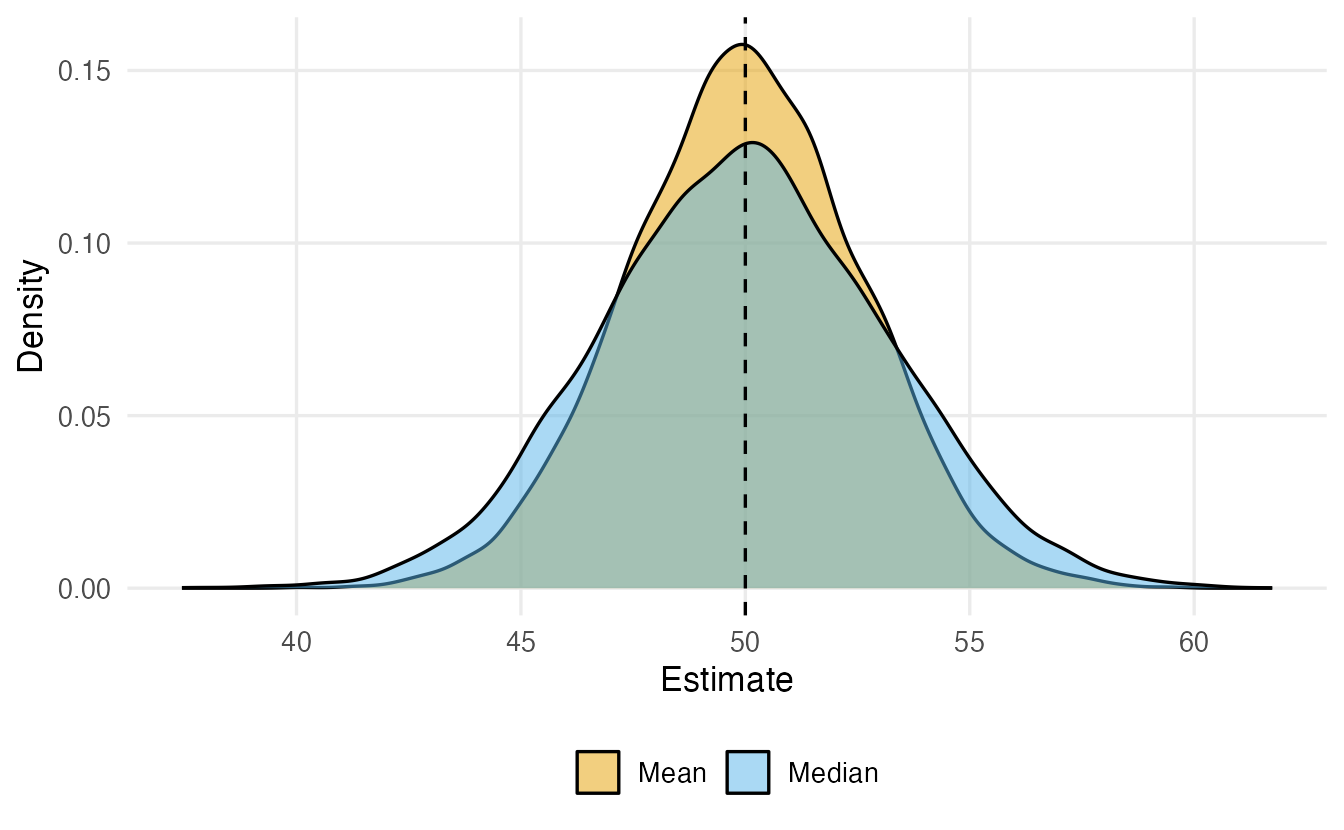

Figure 5: Sampling distributions of the sample mean and sample median (n = 15, normal population with μ = 50). Both are centred on 50; the median is more spread out.

Both are (essentially) unbiased, but for normal data the median’s SE is about 1.23 times larger: the mean uses the information in the data more efficiently. The median’s advantage is robustness: one wild outlier barely moves it (see Summary statistics). With heavy-tailed or contaminated data the comparison can flip.

Why the sample variance divides by \(n - 1\)

You may have wondered why var() and sd() divide by \(n - 1\) rather than \(n\). Simulation gives the answer. Draw many samples of size 5 from a population with variance \(\sigma^2 = 4\) and compare both divisors:

set.seed(7)
n <- 5
vars <- replicate(10000, {
  x <- rnorm(n, mean = 0, sd = 2)               # true variance = 4
  ss <- sum((x - mean(x))^2)                    # sum of squared deviations
  c(divide_by_n = ss / n, divide_by_n_minus_1 = ss / (n - 1))
})
rowMeans(vars)

#>         divide_by_n divide_by_n_minus_1 
#>               3.212               4.015

var_df <- data.frame(
  estimate = c(vars[1, ], vars[2, ]),
  divisor = rep(c("n", "n - 1"), each = ncol(vars))
)
avg_df <- data.frame(divisor = c("n", "n - 1"), avg = rowMeans(vars))
ggplot(var_df, aes(estimate, fill = divisor)) +
  geom_histogram(bins = 60, alpha = 0.5, position = "identity") +
  geom_vline(xintercept = 4, linetype = "dashed") +
  geom_point(data = avg_df, aes(x = avg, y = 0, colour = divisor),
             size = 4, inherit.aes = FALSE) +
  coord_cartesian(xlim = c(0, 16)) +
  labs(x = "Estimated variance", y = "Number of samples",
       fill = "Divisor", colour = "Divisor")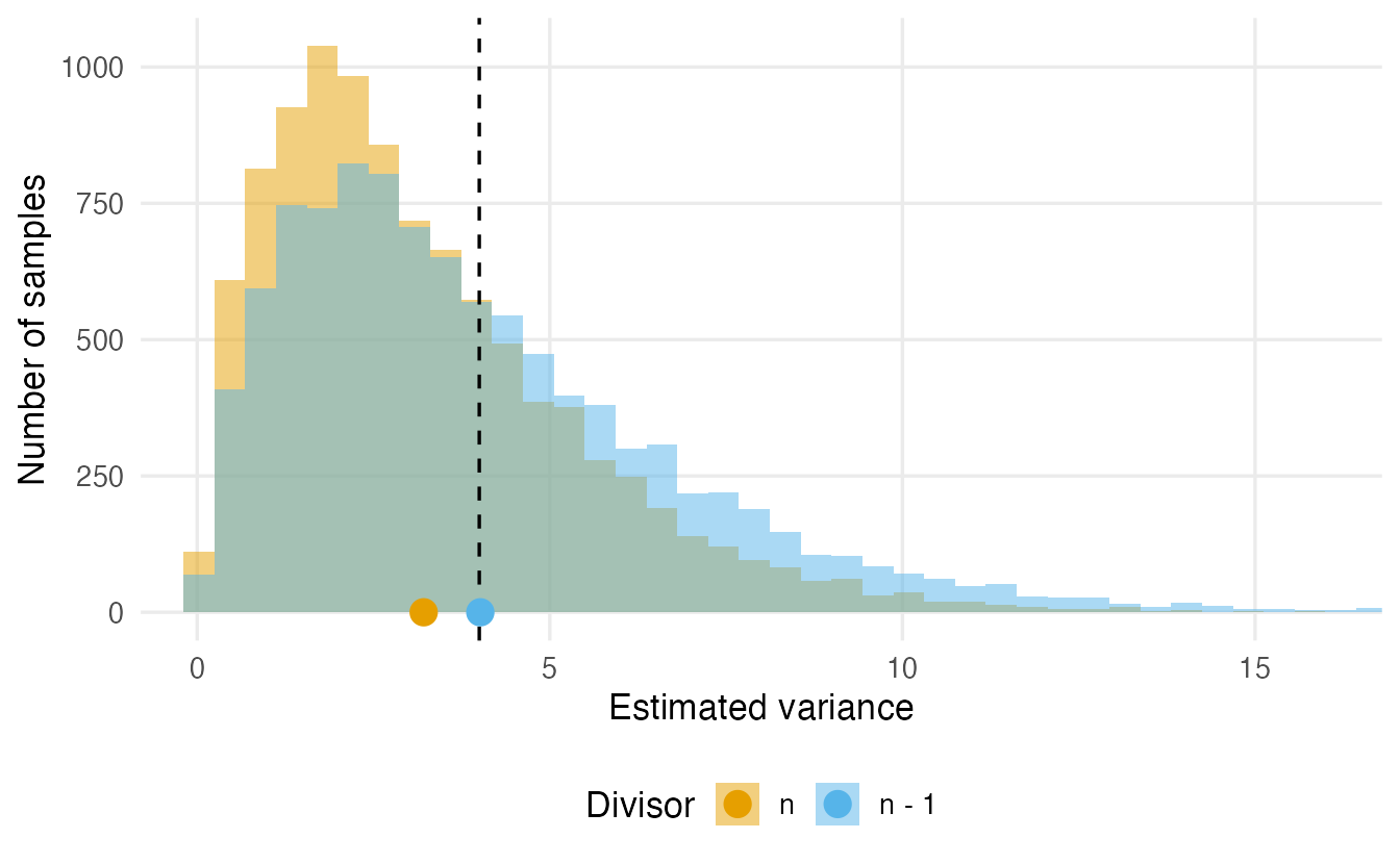

Figure 6: Sampling distributions of the variance estimate with divisor n and n − 1 (n = 5, true variance 4, dashed). Points mark the average of each estimator: only the n − 1 version is centred on the truth.

Dividing by \(n\) gives estimates that are too small on average (about 3.21 instead of 4). The reason: deviations are measured from the sample mean \(\bar x\), which sits in the middle of the sample by construction, so the data look less spread out than they really are around \(\mu\). Dividing by \(n - 1\) exactly corrects this. The \(n - 1\) is called the degrees of freedom: once \(\bar x\) is fixed, only \(n - 1\) deviations are free to vary.

NoteGoing deeper: the bias of the divisor-\(n\) variance

With \(S_n^2 = \frac1n \sum (X_i - \bar X)^2\) one can show \(E(S_n^2) = \frac{n-1}{n}\sigma^2\). For \(n = 5\) this is \(0.8 \times 4 = 3.2\), matching the simulation. Hence \(s^2 = \frac{1}{n-1}\sum (X_i - \bar X)^2\) satisfies \(E(s^2) = \sigma^2\). The bias vanishes as \(n\) grows, so it matters most for small samples. (Curiously, \(s = \sqrt{s^2}\) is still slightly biased for \(\sigma\); unbiasedness does not survive non-linear transformations.)

7. The sampling distribution of a proportion

Many questions are about proportions: the share of voters supporting a candidate, the share of patients who recover. Suppose 30% of a large population supports a proposal (\(p = 0.3\)) and a poll asks \(n = 50\) people. The number of supporters in the sample is \(\text{Binomial}(50, 0.3)\) (see Probability distributions), so we can simulate many polls directly:

set.seed(8)
p <- 0.3
n_poll <- 50
p_hat <- rbinom(10000, size = n_poll, prob = p) / n_poll
c(mean = mean(p_hat), simulated_se = sd(p_hat),
  formula_se = sqrt(p * (1 - p) / n_poll))

#>         mean simulated_se   formula_se 
#>      0.30014      0.06543      0.06481

The sample proportion \(\hat p\) is unbiased for \(p\) and its standard error is

\[ \operatorname{SE}(\hat p) = \sqrt{\frac{p(1-p)}{n}} . \]

A proportion is the mean of 0/1 values, so the CLT applies: for large enough \(n\) the distribution of \(\hat p\) is approximately normal.

set.seed(9)
prop_df <- do.call(rbind, lapply(c(10, 50, 500), \(m) {
  data.frame(n = m, p_hat = rbinom(10000, m, p) / m)
}))
curve_df <- do.call(rbind, lapply(c(10, 50, 500), \(m) {
  se <- sqrt(p * (1 - p) / m)
  x <- seq(0, 0.8, length.out = 300)
  data.frame(n = m, p_hat = x, density = dnorm(x, p, se))
}))
ggplot(prop_df, aes(p_hat)) +
  geom_histogram(aes(y = after_stat(density)), binwidth = 0.01,
                 fill = "#CC79A7", colour = "white") +
  geom_line(data = curve_df, aes(y = density), linewidth = 0.9) +
  facet_wrap(~ n, ncol = 1, scales = "free_y", labeller = label_both) +
  labs(x = "Sample proportion", y = "Density")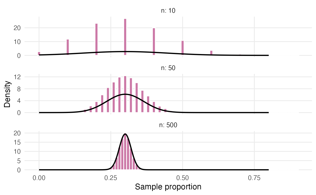

Figure 7: Sampling distribution of a sample proportion (p = 0.3) for polls of 10, 50 and 500 people, with the normal approximation from the CLT (curve). The approximation is rough for n = 10 and very good for n = 500.

A common rule of thumb for the normal approximation is to have at least about 10 expected “successes” and 10 “failures” (\(np \ge 10\) and \(n(1-p) \ge 10\)).

8. From sampling distributions to inference

Everything so far assumed we know the population. Real inference runs the logic backwards. Because the sampling distribution of \(\bar x\) is approximately normal with SD equal to the SE, about 95% of all samples produce a mean within \(1.96\) SE of \(\mu\):

se_25 <- sigma / sqrt(25)
mean(abs(means_25 - mu) < 1.96 * se_25)

#> [1] 0.9506

Turn this sentence around: if 95% of sample means fall within 1.96 SE of \(\mu\), then for 95% of samples \(\mu\) lies within 1.96 SE of the sample mean. That is a 95% confidence interval, \(\bar x \pm 1.96\,\text{SE}\), the subject of Confidence intervals.

And if someone claims that \(\mu = 12\) minutes, we can ask whether our observed mean is unusually far from 12 in units of SE. That is the logic of a hypothesis test, developed in Hypothesis testing. In both cases, the sampling distribution is the yardstick.

But what if the statistic has no simple SE formula (a median, a correlation) and we have only one sample? The next lesson shows how to estimate a sampling distribution from the sample itself.

WarningCommon pitfalls

1. Confusing the three distributions. The population distribution (all units), the sample distribution (the data you have) and the sampling distribution (a statistic over many hypothetical samples) are different things. The CLT is about the third.
2. Using the SD when you mean the SE, or vice versa. Error bars must say which one they show.
3. “The CLT makes my data normal.” It does not. It describes averages of many observations, and it needs independent observations.
4. Treating n = 30 as magic. For strongly skewed populations (incomes, reaction times, insurance claims) the mean may still be far from normal at n = 30.
5. Believing that a larger population requires a larger sample. Precision depends on \(n\) (and on randomness of the sample), not on the population size.
6. Equating “unbiased” with “good”. An unbiased estimator can be very imprecise; a slightly biased one with a much smaller SE can be preferable (a trade-off we will meet again in Penalized regression).

9. Check your understanding

NoteQ1. A sample of 100 has SE = 4 for the mean. Approximately what SE would a sample of 400 from the same population have?

About 2. Multiplying \(n\) by 4 divides the SE by \(\sqrt 4 = 2\).

NoteQ2. Is the sample mean \(\bar x\) a parameter or a statistic? And \(\mu\)?

\(\bar x\) is a statistic: it is computed from the sample and changes from sample to sample. \(\mu\) is a parameter: a fixed (usually unknown) property of the population.

NoteQ3. The incomes in a city are strongly right-skewed. What does the CLT say about (a) the distribution of incomes in a random sample of 500 people, (b) the distribution of the sample mean income across many such samples?

1. Nothing: the sample will be right-skewed like the population. (b) The sample mean, over many samples, will be approximately normal (with \(n = 500\), even for quite skewed data), centred on the population mean with SD \(\sigma/\sqrt{500}\).

NoteQ4. Why does var() divide by \(n - 1\)?

Because deviations are measured from the sample mean, which makes the sum of squares systematically too small; dividing by \(n - 1\) instead of \(n\) makes the estimator unbiased for the population variance.

10. Exercises

Interactive (run in your browser)

★ Exercise 1 — penguins as a population. Pretend the 342 penguins with a recorded body mass are the entire population. Compute the population mean, then simulate 5,000 samples of 20 penguins and compare (a) the mean of the sample means with \(\mu\) and (b) the SD of the sample means with \(\sigma/\sqrt{20}\).

All three blanks involve the sample size 20 or the vector xbars.

mass <- penguins$body_mass[!is.na(penguins$body_mass)]
mu <- mean(mass)
sigma <- sd(mass)
set.seed(1)
xbars <- replicate(5000, mean(sample(mass, size = 20)))
c(mu = mu, mean_of_means = mean(xbars))
c(simulated_se = sd(xbars), formula_se = sigma / sqrt(20))

The means are centred on \(\mu \approx 4202\) g and their SD is about 172 g, close to \(\sigma/\sqrt{20} \approx 179\) g. (The simulated SE is slightly smaller because we sample without replacement from a small population of 342: the finite-population correction from the “Going deeper” box.)

★★ Exercise 2 — predict, then simulate. Using the mass population from Exercise 1, the SE for \(n = 5\) is about 360 g. Predict the SE for \(n = 20\) and \(n = 80\) before running the code. Note that we now sample with replacement, so the \(\sigma/\sqrt n\) formula holds exactly.

Use replace = TRUE and apply se_for to each sample size. Each fourfold increase in \(n\) should halve the SE.

se_for <- function(n) {
  sd(replicate(5000, mean(sample(mass, n, replace = TRUE))))
}
sapply(c(5, 20, 80), se_for)   # roughly 360, 180, 90

The SE halves each time \(n\) is multiplied by four: \(\sigma/\sqrt 5 \approx 359\), \(\sigma/\sqrt{20} \approx 179\), \(\sigma/\sqrt{80} \approx 90\).

★★★ Exercise 3 — when is n “large enough”? A log-normal population (rlnorm(n, sdlog = 1.5)) is extremely right-skewed, like incomes or insurance claims. Draw histograms of 5,000 sample means for \(n = 5\), \(30\) and \(200\). Is \(n = 30\) enough for the CLT here?

The sample size inside rlnorm() is the loop variable n.

set.seed(3)
par(mfrow = c(1, 3))
for (n in c(5, 30, 200)) {
  xbar <- replicate(5000, mean(rlnorm(n, sdlog = 1.5)))
  hist(xbar, breaks = 50, main = paste("n =", n), xlab = "Sample mean")
}
par(mfrow = c(1, 1))

At \(n = 30\) the distribution of the mean is still clearly right-skewed (its skewness is still around 3), and even at \(n = 200\) a long right tail remains. For very skewed populations the CLT needs much larger samples, or a different summary (such as the median or the mean of the log values).

★★ Exercise 4 — a proportion. In a population, 10% of people are left-handed. Simulate 10,000 samples of size 20 and of size 200, compute the sample proportion of left-handers in each, and compare the simulated SE with \(\sqrt{p(1-p)/n}\). For which \(n\) is a normal approximation reasonable?

Divide the counts by n; the formula is sqrt(p * (1 - p) / n). Then try hist(p_hat) for each n, and check the rule of thumb \(np \ge 10\).

p <- 0.1
set.seed(4)
for (n in c(20, 200)) {
  p_hat <- rbinom(10000, size = n, prob = p) / n
  cat("n =", n, " simulated SE =", round(sd(p_hat), 4),
      " formula SE =", round(sqrt(p * (1 - p) / n), 4), "\n")
}

The SEs are about 0.067 for \(n = 20\) and 0.021 for \(n = 200\), matching the formula. With \(n = 20\) we expect only \(np = 2\) left-handers: the distribution of \(\hat p\) is lumpy and right-skewed, and the normal approximation is poor. With \(n = 200\) (\(np = 20\)) it is good.

Practice on your own computer

★★ Exercise 5 — how much does \(n - 1\) matter? Repeat the variance-divisor simulation of Section 6 for \(n = 2, 5, 20\) and \(100\) (true variance 4). For each \(n\), report the average of the divisor-\(n\) estimates and compare it with \(\frac{n-1}{n} \times 4\). When can you stop worrying about the difference?

TipSolution

set.seed(10)
avg_biased <- sapply(c(2, 5, 20, 100), \(n) {
  mean(replicate(10000, {
    x <- rnorm(n, sd = 2)
    sum((x - mean(x))^2) / n
  }))
})
data.frame(n = c(2, 5, 20, 100), average = avg_biased,
           theory = (c(2, 5, 20, 100) - 1) / c(2, 5, 20, 100) * 4)

The divisor-\(n\) estimator averages about 2, 3.2, 3.8 and 3.96: half the true variance at \(n = 2\), but only 1% too small at \(n = 100\). The correction matters for small samples and becomes negligible for large ones.

Summary

Idea	Formula / code	Meaning
Parameter vs statistic	\(\mu\) vs \(\bar x\), \(p\) vs \(\hat p\)	Fixed truth vs value computed from a sample
Sampling distribution	replicate(B, stat(sample(pop, n)))	Distribution of a statistic over many samples
Standard error of the mean	\(\sigma/\sqrt n\), estimated by sd(x) / sqrt(n)	Typical distance between estimate and parameter
Standard error of a proportion	\(\sqrt{p(1-p)/n}\)	Same, for \(\hat p\)
Central Limit Theorem	\(\bar X \approx N(\mu, \sigma/\sqrt n)\) for large \(n\)	Means are approximately normal, whatever the data
Unbiased estimator	centre of sampling distribution = parameter	Right on average; var() uses \(n - 1\) for this

• Every estimate is one draw from its sampling distribution; a different sample would give a different number.
• The standard error measures the precision of an estimate and shrinks like \(1/\sqrt n\): four times the data, half the error.
• The CLT makes sample means approximately normal for large \(n\) — the foundation of confidence intervals and tests.
• Unbiased means “right on average”; precision is a separate property.

NoteFurther reading

• Çetinkaya-Rundel & Hardin, Introduction to Modern Statistics (2e), chapters on foundations of inference, https://openintro-ims.netlify.app
• Diez, Çetinkaya-Rundel & Barr, OpenIntro Statistics (free PDF), https://www.openintro.org/book/os/
• Wickham, Çetinkaya-Rundel & Grolemund, R for Data Science (2e), https://r4ds.hadley.nz