Summary statistics
Centre, spread, position and shape — a distribution in a few numbers
Summarise a numeric variable with measures of location (mean, median, trimmed mean), spread (range, IQR, variance, SD), position (quantiles), shape (skewness), z-scores and the coefficient of variation, overall and by group.
NoteLearning objectives
By the end of this lesson you will be able to:
- compute and interpret the mean, median, mode and trimmed mean, and explain which are robust to outliers;
- measure spread with the range, IQR, variance and standard deviation, and explain what the SD measures;
- use quantiles and z-scores to describe the position of a value;
- describe the shape of a distribution (skewness) and use mean vs median as a quick indicator;
- produce summaries by group and the five-number summary behind a boxplot.
library(dplyr)
library(ggplot2)
1. Why summarise?
A frequency table or a histogram shows a whole distribution. Often, though, we need to compress it into a few numbers: to compare species, to write a report, or to feed a later analysis. A good summary answers four questions:
| Question | Family of statistics | Examples |
|---|---|---|
| Where is the centre? | Location | mean, median, mode |
| How spread out are the values? | Spread (dispersion) | range, IQR, variance, standard deviation |
| Where does a particular value stand? | Position | quantiles, percentiles, z-scores |
| What shape does the distribution have? | Shape | skewness |
No single number answers all four. Throughout the lesson we use the body mass (in grams) of the penguins. Many functions need na.rm = TRUE, because body_mass has 2 missing values; to keep the code short we create a vector without them:
mass <- penguins$body_mass[!is.na(penguins$body_mass)]
length(mass)
#> [1] 3422. Location: where is the centre?
Mean and median
The mean (average) adds all values and divides by how many there are. The median is the middle value once the data are sorted: half of the observations are below it and half above.
mean(mass)#> [1] 4202median(mass)#> [1] 4050The mean is the balance point of the data: if each penguin were a weight placed on a ruler at its body mass, the ruler would balance at the mean. The median is the halfway point by count. Here the mean (4202 g) is a bit larger than the median (4050 g); Section 5 explains why.
Robustness: what happens with an outlier?
Suppose that while typing the data someone enters 37500 instead of 3750 for the first bird — a single typo among 342 values.
mass_typo <- mass
mass_typo[1] <- 37500

c(mean_clean = mean(mass), mean_typo = mean(mass_typo))
#> mean_clean mean_typo
#> 4202 4300c(median_clean = median(mass), median_typo = median(mass_typo))#> median_clean median_typo
#> 4050 4050One wrong value moved the mean by about 99 g, while the median did not move at all. A statistic that is barely affected by a few extreme values is called robust. The median is robust; the mean is not.
Trimmed mean
The trimmed mean is a compromise: it removes a fixed percentage of the smallest and largest values and averages the rest.
c(trim10_clean = mean(mass, trim = 0.1),
  trim10_typo  = mean(mass_typo, trim = 0.1))
#> trim10_clean trim10_typo
#> 4154 4160trim = 0.1 drops the lowest 10% and the highest 10%. The typo now changes the result by only a few grams.
Mode
For numeric data the mode (most frequent value) is useful only for discrete variables with few distinct values, such as the number of gears in mtcars (see Frequency tables). For a continuous variable almost every value is unique, so the mode depends on rounding and is rarely reported.
NoteGoing deeper: what each “centre” minimises
For data \(x_1, \dots, x_n\):
- the mean \(\bar x = \frac1n\sum_i x_i\) is the value \(c\) that minimises the sum of squared distances \(\sum_i (x_i - c)^2\);
- the median is the value \(c\) that minimises the sum of absolute distances \(\sum_i |x_i - c|\).
Squaring gives large distances a big weight, which is why one far-away value can drag the mean. The breakdown point formalises robustness: it is the fraction of observations that can be made arbitrarily bad before the statistic becomes arbitrarily bad. It is \(0\) for the mean (one value is enough), 50% for the median and equal to the trimming fraction for a trimmed mean.
3. Spread: how different are the values?
Two groups can have the same centre and still be very different. Spread measures how far the values typically are from each other.
Range and IQR
range(mass) # minimum and maximum#> [1] 2700 6300diff(range(mass)) # the range as a single number#> [1] 3600IQR(mass) # interquartile range = Q3 - Q1#> [1] 1200The range depends only on the two most extreme values, so it is very sensitive to outliers and tends to grow with the sample size. The interquartile range (IQR) is the width of the middle 50% of the data (from the first quartile Q1 to the third quartile Q3, see Section 4). It is robust.
Variance and standard deviation: the intuition
The most used measure of spread is the standard deviation (SD). Think of it as “the typical distance of an observation from the mean”. Let us build it on five small numbers:
x <- c(2, 4, 4, 5, 9)
dev <- x - mean(x)          # deviations from the mean
dev
#> [1] -2.8 -0.8 -0.8 0.2 4.2sum(dev) # always 0: positives and negatives cancel#> [1] 8.882e-16sum(dev^2) / (length(x) - 1) # variance#> [1] 6.7var(x)#> [1] 6.7sqrt(var(x)) # standard deviation#> [1] 2.588sd(x)#> [1] 2.588
TipHow to read this output
- The deviations say how far each value is from the mean (4.8), with a sign.
- They always add up to 0, so their plain average is useless. Squaring makes them all positive.
- The variance is (almost) the average squared deviation. Its unit is “squared units” (g² for body mass), which is hard to interpret.
- The standard deviation is the square root of the variance, so it is back in the original units. Here a typical value is about 2.6 away from the mean.
For the penguins:
c(var = var(mass), sd = sd(mass))#> var sd
#> 643131 802c(sd_clean = sd(mass), sd_typo = sd(mass_typo))#> sd_clean sd_typo
#> 802 1971A typical penguin’s mass is about 802 g away from the average. But the SD is not robust: the single typo more than doubles it, while the IQR barely changes (1200 vs 1218.75). A robust alternative to the SD is the median absolute deviation, mad().
NoteGoing deeper: why divide by \(n-1\)?
The sample variance is
\[ s^2 = \frac{1}{n-1}\sum_{i=1}^n (x_i - \bar x)^2 . \]
We would like to know the spread around the true population mean \(\mu\), but we only know the sample mean \(\bar x\). Because \(\bar x\) is computed from the same data, it is always “closer” to the data than \(\mu\) is (it minimises the sum of squares). So \(\sum (x_i - \bar x)^2\) is on average a bit too small, and dividing by \(n - 1\) instead of \(n\) corrects exactly for that. Equivalently, once \(\bar x\) is fixed only \(n-1\) deviations are free (they must sum to 0): we have \(n - 1\) degrees of freedom.
A simulation shows the effect. We draw many samples of size 5 from a population with SD \(= 10\) (variance \(= 100\)):
set.seed(2026)
sims <- replicate(10000, {
  x <- rnorm(5, mean = 0, sd = 10)
  c(divide_n = sum((x - mean(x))^2) / 5, divide_n1 = var(x))
})
rowMeans(sims)
#> divide_n divide_n1
#> 80.05 100.06Dividing by \(n\) gives on average about 80 — it underestimates 100 by the factor \((n-1)/n = 0.8\). Dividing by \(n - 1\) is right on average (it is unbiased). With large \(n\) the difference is negligible.
4. Position: quantiles, percentiles and z-scores
Quantiles
The \(p\)-quantile is the value below which a proportion \(p\) of the data lies. Percentiles are quantiles expressed in percent; the quartiles split the data into four parts (Q1 = 25th percentile, Q2 = median, Q3 = 75th percentile).
quantile(mass) # min, Q1, median, Q3, max#> 0% 25% 50% 75% 100%
#> 2700 3550 4050 4750 6300quantile(mass, probs = c(0.1, 0.9)) # 10th and 90th percentiles#> 10% 90%
#> 3300 540010% of the penguins weigh 3300 g or less; 90% weigh 5400 g or less. The opposite question — “what percentage of birds weigh at most 5000 g?” — is answered by a proportion:
mean(mass <= 5000)#> [1] 0.8216(mass <= 5000 is a logical vector and the mean of TRUE/FALSE values is the proportion of TRUE.)
NoteGoing deeper: there are nine ways to compute a quantile
With a finite sample, the 25th percentile often falls between two observations, and there are several reasonable rules for interpolating. quantile() implements nine of them through the type argument; R’s default is type = 7, SAS and SPSS use type = 6, and Hyndman & Fan (1996) recommend type = 8. For six numbers they really differ:
small <- c(1, 3, 4, 8, 10, 15)
sapply(c(6, 7, 8), \(t) quantile(small, 0.25, type = t))
#> 25% 25% 25%
#> 2.500 3.250 2.833For hundreds of observations the differences are tiny, but they explain why two programs can report slightly different quartiles for the same data.
z-scores and standardisation
Is a 4500 g penguin heavy? It depends on the species. The z-score expresses a value as the number of standard deviations above (+) or below (−) the mean:
\[ z = \frac{x - \bar x}{s}. \]
penguins |>
  filter(!is.na(body_mass)) |>
  mutate(z = (body_mass - mean(body_mass)) / sd(body_mass),
         .by = species) |>
  filter(body_mass == 4500) |>
  select(species, body_mass, z)
#> species body_mass z
#> 1 Adelie 4500 1.743
#> 2 Gentoo 4500 -1.143
#> 3 Chinstrap 4500 1.995The same 4500 g is far above average for an Adelie or Chinstrap penguin, and well below average for a Gentoo. Because .by = species, each bird is standardised against its own species. After standardisation every variable has mean 0 and SD 1, whatever its original unit: z-scores let us compare things measured on different scales.
The function scale() standardises too, but it returns a matrix, which is awkward inside a data frame. Use as.numeric(scale(x)), or write the formula as above.
z_mass <- as.numeric(scale(mass))
c(mean = mean(z_mass), sd = sd(z_mass))
#> mean sd
#> 9.187e-17 1.000e+00mean(abs(z_mass) <= 2)#> [1] 0.9737For roughly bell-shaped data about 95% of the values have \(|z| \le 2\); here the proportion is 0.974. A value with \(|z| > 3\) is unusual and worth checking. (The “95%” is a property of the normal distribution, see Distributions; for strongly skewed data it does not hold.)
5. Shape: symmetric or skewed?
The shape of a distribution describes how the values are arranged around the centre. A distribution is symmetric if its left and right halves are mirror images. It is right-skewed (positively skewed) if it has a long tail towards large values and left-skewed (negatively skewed) if the long tail points to small values.
shape_df <- bind_rows(
  tibble(variable = "Gentoo body mass (g)",
         value = penguins$body_mass[penguins$species == "Gentoo"]),
  tibble(variable = "Ozone (ppb)", value = airquality$Ozone),
  tibble(variable = "Solar radiation (lang)", value = airquality$Solar.R)
) |>
  filter(!is.na(value))

centres <- shape_df |>
  summarise(mean = mean(value), median = median(value), .by = variable)

ggplot(shape_df, aes(value)) +
  geom_histogram(bins = 20, fill = "grey70", colour = "white") +
  geom_vline(data = centres, aes(xintercept = mean), linetype = "dashed") +
  geom_vline(data = centres, aes(xintercept = median)) +
  facet_wrap(~ variable, scales = "free") +
  labs(x = NULL, y = "Count")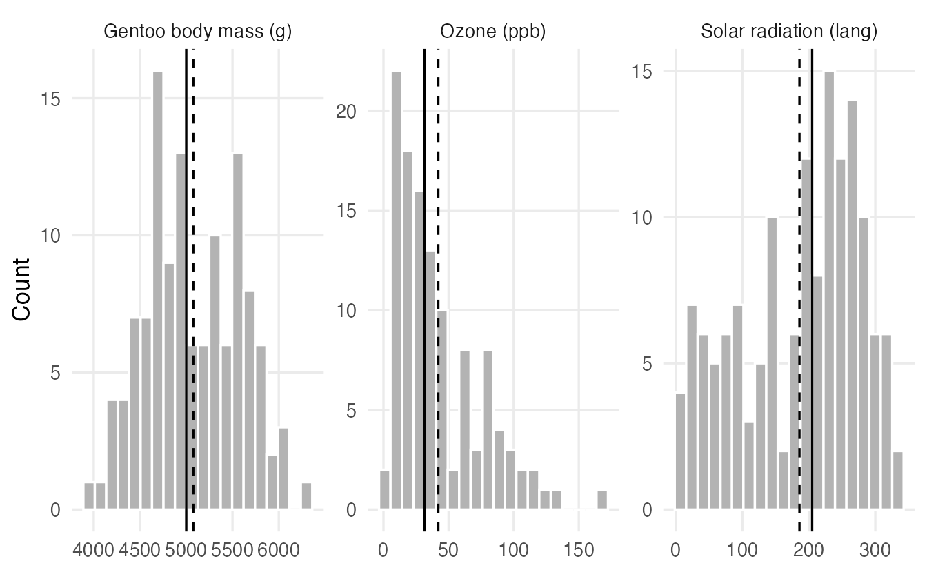
Mean vs median as a quick indicator
The mean is pulled towards the long tail; the median is not. So:
- mean ≈ median → roughly symmetric;
- mean > median → right-skewed (typical for incomes, waiting times, concentrations);
- mean < median → left-skewed.
centres#> # A tibble: 3 × 3
#> variable mean median
#> <chr> <dbl> <dbl>
#> 1 Gentoo body mass (g) 5076. 5000
#> 2 Ozone (ppb) 42.13 31.5
#> 3 Solar radiation (lang) 185.9 205For Ozone the mean is 42.1 and the median only 31.5: a few very polluted days pull the mean up. For a skewed variable the median usually describes a “typical” value better.
A number for skewness
The sample skewness averages the cubed z-scores. Cubing keeps the sign, so long right tails give large positive values and long left tails large negative values; in a symmetric distribution they cancel out.
skewness <- function(x) {
  x <- x[!is.na(x)]
  m <- mean(x)
  mean((x - m)^3) / mean((x - m)^2)^(3 / 2)
}

c(gentoo_mass = skewness(penguins$body_mass[penguins$species == "Gentoo"]),
  ozone       = skewness(airquality$Ozone),
  solar       = skewness(airquality$Solar.R))
#> gentoo_mass ozone solar
#> 0.06878 1.22568 -0.42363As a rough guide, values between −0.5 and 0.5 indicate approximate symmetry and values beyond ±1 strong skewness. Always look at the plot as well: a single number cannot tell you, for example, that a distribution has two peaks.
NoteGoing deeper: moments, skewness and kurtosis
The function above computes
\[ g_1 = \frac{\frac1n\sum_i (x_i - \bar x)^3}{\left(\frac1n\sum_i (x_i - \bar x)^2\right)^{3/2}} , \]
the third central moment divided by the second raised to \(3/2\). Packages such as e1071 or moments offer this and slightly different, bias-adjusted versions (they differ noticeably only for small \(n\)). The fourth standardised moment, kurtosis, describes how heavy the tails are compared with a normal distribution (whose kurtosis is 3; “excess kurtosis” subtracts 3).
6. Relative spread: the coefficient of variation
Is body mass more variable than bill length? Their SDs (802 g vs 5.5 mm) cannot be compared: different units. The coefficient of variation (CV) divides the SD by the mean, giving a unit-free relative spread:
cv <- function(x) sd(x, na.rm = TRUE) / mean(x, na.rm = TRUE)
c(body_mass = cv(penguins$body_mass), bill_len = cv(penguins$bill_len),
  flipper_len = cv(penguins$flipper_len))
#> body_mass bill_len flipper_len
#> 0.19086 0.12430 0.06999Body mass varies about 19% around its mean, flipper length only about 7%. The CV makes sense only for variables measured on a ratio scale (with a true zero and only positive values, like mass or length). It is meaningless for temperatures in °C or for z-scores, whose mean can be 0 or negative.
7. Everything at once: summary() and grouped summaries
summary() gives the minimum, quartiles, mean, maximum and the number of NAs for every numeric column (and counts for factors):
summary(penguins[, c("species", "bill_len", "body_mass")])#> species bill_len body_mass
#> Adelie :152 Min. :32.1 Min. :2700
#> Chinstrap: 68 1st Qu.:39.2 1st Qu.:3550
#> Gentoo :124 Median :44.5 Median :4050
#> Mean :43.9 Mean :4202
#> 3rd Qu.:48.5 3rd Qu.:4750
#> Max. :59.6 Max. :6300
#> NAs :2 NAs :2Overall summaries can hide very different groups. Combine summarise() with .by (see Grouped summaries):
penguins |>
  filter(!is.na(body_mass)) |>
  summarise(
    n      = n(),
    mean   = mean(body_mass),
    median = median(body_mass),
    sd     = sd(body_mass),
    iqr    = IQR(body_mass),
    cv     = sd / mean,
    .by = species
  )
#> species n mean median sd iqr cv
#> 1 Adelie 151 3701 3700 458.6 650.0 0.12391
#> 2 Gentoo 123 5076 5000 504.1 800.0 0.09931
#> 3 Chinstrap 68 3733 3700 384.3 462.5 0.10295
TipHow to read this output
- Gentoo penguins are about 1.3–1.4 kg heavier than the other two species, which have similar centres.
- Within each species mean and median are close: the groups are roughly symmetric. The overall right skew of
body_masscomes mostly from mixing a heavy species with two lighter ones. - The SDs are of similar size, and so are the CVs (around 10–12%).
- Always report
nwith group summaries: a mean based on 5 birds deserves less trust than one based on 150.
8. The five-number summary: a bridge to boxplots
The five-number summary — minimum, Q1, median, Q3, maximum — describes centre, spread and (roughly) shape in five numbers. fivenum() computes it with Tukey’s definition of the quartiles (“hinges”), which can differ slightly from quantile():
fivenum(airquality$Ozone)#> [1] 1.0 18.0 31.5 63.5 168.0quantile(airquality$Ozone, na.rm = TRUE)#> 0% 25% 50% 75% 100%
#> 1.00 18.00 31.50 63.25 168.00(Q3 is 63.5 with fivenum() and 63.25 with quantile(): two conventions, as in the quantile box above.)
The boxplot is a drawing of the five-number summary, with a rule for flagging unusual values: points more than 1.5 × IQR beyond the box are shown individually.
ggplot(airquality, aes(x = Ozone, y = "")) +
  geom_boxplot(na.rm = TRUE) +
  labs(x = "Ozone (ppb)", y = NULL)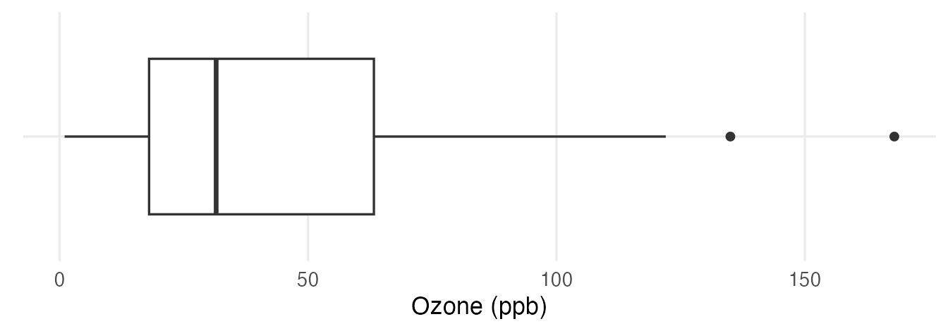
You will learn to read every part of it in Distribution plots.
WarningCommon pitfalls
- Forgetting
na.rm = TRUE.mean(penguins$body_mass)returnsNA. The missing values are not ignored automatically — and that is a feature: R forces you to notice them. - Reporting only the mean for skewed data. For incomes, waiting times or concentrations, report the median (and IQR) as well, or instead.
- Reading the SD as the “maximum distance” or the “range”. It is a typical distance from the mean; many values are farther away than one SD.
- Using
scale()insidemutate()withoutas.numeric(). It returns a one-column matrix with attributes, which can cause surprising behaviour later. - Comparing SDs of variables measured in different units. Use z-scores or the coefficient of variation (for ratio-scale variables).
- Trusting a summary without a plot. Very different distributions can share the same mean and SD (you will see a dramatic example in Correlation).
9. Check your understanding
10. Exercises
Interactive (run in your browser)
★ Exercise 1 — centre and spread of mpg. Compute the mean, median, SD and IQR of fuel consumption (mpg) in mtcars. Is the distribution symmetric or skewed?
The functions are mean(), median(), sd() and IQR().
x <- mtcars$mpg
c(mean = mean(x), median = median(x), sd = sd(x), iqr = IQR(x))
The mean (about 20.1) is larger than the median (19.2): a mild right skew — a few very economical cars make the right tail longer.
★★ Exercise 2 — predict, then check. Before running the code, predict which numbers will change when the largest hp value in mtcars is multiplied by 10. Then run it.
Pass hp2 to stats(). Which statistics use the values of the extremes, and which only their position in the sorted data?
rbind(original = stats(hp), changed = stats(hp2))The mean and especially the SD change a lot; the median, the IQR and the 10% trimmed mean do not change at all, because the modified car is in the top 10% that gets trimmed and it stays the largest value.
★★ Exercise 3 — grouped summary. Using dplyr, compute for each species the number of birds with a known flipper length, the mean, the median and the SD of flipper_len. Which species has the longest flippers on average?
Use n(), mean(flipper_len), median(flipper_len), sd(flipper_len) and .by = species.
penguins |>
  filter(!is.na(flipper_len)) |>
  summarise(n = n(), mean = mean(flipper_len),
            median = median(flipper_len), sd = sd(flipper_len),
            .by = species)
Gentoo penguins have by far the longest flippers (mean about 217 mm, versus about 190 mm for Adelie and 196 mm for Chinstrap). Within each species mean and median are close.
★★★ Exercise 4 — z-scores across variables. The car "Maserati Bora" in mtcars: is it more extreme in horsepower (hp) or in weight (wt)? Compare z-scores.
Index the z-score vectors with i: z_hp[i].
c(hp = z_hp[i], wt = z_wt[i])Its horsepower is about 2.7 SDs above the mean, its weight only about 0.4 SD above: it is far more unusual in power than in weight. z-scores make variables measured in different units comparable.
Practice on your own computer
★★ Exercise 5 — shape of airquality variables. Using the skewness() function from Section 5, compute the skewness of Ozone, Solar.R, Wind and Temp. For each, compare the mean with the median and draw a histogram. Do the three indicators (number, mean vs median, picture) agree?
TipSolution
vars <- c("Ozone", "Solar.R", "Wind", "Temp")
sapply(airquality[vars], skewness)
sapply(airquality[vars], \(v) c(mean = mean(v, na.rm = TRUE),
                                median = median(v, na.rm = TRUE)))

ggplot(airquality, aes(Temp)) +
  geom_histogram(bins = 15) +
  labs(x = "Temperature (°F)", y = "Count")
Ozone is strongly right-skewed (skewness about 1.2, mean ≈ 42 > median 31.5). Solar.R is moderately left-skewed (about −0.4, mean < median). Wind (about 0.3) and Temp (about −0.4) are mildly skewed. The three indicators agree on the direction.
★★★ Exercise 6 — your own summary function. Write a function describe(x) that returns, as a named vector, n (non-missing), mean, sd, min, q1, median, q3, max and skew. Apply it to every numeric column of penguins with sapply(), and to body_mass for each species with tapply().
TipSolution
describe <- function(x) {
  x <- x[!is.na(x)]
  q <- quantile(x, c(0.25, 0.5, 0.75))
  c(n = length(x), mean = mean(x), sd = sd(x), min = min(x),
    q1 = q[[1]], median = q[[2]], q3 = q[[3]], max = max(x),
    skew = skewness(x))
}

num_cols <- c("bill_len", "bill_dep", "flipper_len", "body_mass")
round(sapply(penguins[num_cols], describe), 2)
tapply(penguins$body_mass, penguins$species, describe)
Summary
| Idea | R | Robust? |
|---|---|---|
| Mean / trimmed mean | mean(x), mean(x, trim = 0.1) |
No / partly |
| Median | median(x) |
Yes |
| Range, IQR | range(x), IQR(x) |
No, Yes |
| Variance, SD, MAD | var(x), sd(x), mad(x) |
No, No, Yes |
| Quantiles | quantile(x, probs = ); proportion below: mean(x <= v) |
Yes |
| z-scores | (x - mean(x)) / sd(x), as.numeric(scale(x)) |
— |
| Coefficient of variation | sd(x) / mean(x) |
No |
| Skewness | mean((x - m)^3) / mean((x - m)^2)^1.5 |
No |
| Five-number summary | fivenum(x), summary(x) |
Yes |
| By group | summarise(..., .by = g) |
— |
- Describe centre, spread, position and shape — no single number does everything.
- The median and IQR are robust; the mean and SD are sensitive to outliers but are the basis of most of statistics.
- The SD is the typical distance from the mean; we divide by \(n - 1\) to correct for estimating the mean.
- Mean > median suggests right skew; mean < median left skew. Always confirm with a plot.
- Summaries by group often reveal what the overall summary hides.