library(tidymodels)
library(rpart)        # engine for decision trees
library(rpart.plot)   # tree plots

# tidymodels attaches modeldata, whose own `penguins` (with different column
# names) would mask the base-R one: make sure we use R's built-in version.
penguins <- datasets::penguinsDecision trees
Predict by asking a sequence of yes/no questions — and know when to stop asking
How classification and regression trees choose their splits (Gini, entropy, sum of squares), how cost-complexity pruning and the 1-SE rule control their size, how to read them with rpart.plot, how to tune them with tidymodels, and why their instability motivates ensembles.
NoteLearning objectives
By the end of this lesson you will be able to:
- explain how a tree is grown by recursive binary splitting, and compute Gini impurity and entropy by hand for one split;
- grow a regression tree split and explain what it minimises;
- control tree size with cost-complexity pruning and apply the 1-SE rule correctly;
- fit, plot and read a tree with
rpartandrpart.plot, and tune it withdecision_tree()in tidymodels; - show that trees are unstable and explain why this motivates ensembles.
1. Why trees? The “20 questions” game
In the game 20 questions, one player thinks of an object and the other must guess it by asking yes/no questions. Good players ask questions that split the remaining possibilities as cleanly as possible: “Is it alive?” is better than “Is it a toaster?”.
A decision tree predicts in the same way. To predict whether a Titanic passenger survived it might ask: Is the passenger male? If yes: Is he older than 9.5? … Each question splits the passengers into two groups; at the end of each path (a leaf) the tree predicts the majority class (or the class proportions) of the training passengers who ended there.
Trees are attractive because they:
- are easy to explain — a tree with five leaves is a set of five rules;
- capture non-linear effects and interactions automatically (the effect of age can be different for men and women);
- need no scaling of predictors and handle categorical variables naturally.
Their weakness, as we will see, is instability: small changes in the data can produce a very different tree.
We use the same Titanic preparation as in the ML workflow lesson:
titanic <- readr::read_csv(data_path("titanic_data.csv"),
                           na = c("", "NA", "?"), show_col_types = FALSE) |>
  select(survived, pclass, sex, age, sibsp, parch, fare, embarked) |>
  mutate(
    survived = factor(survived, levels = c(1, 0), labels = c("yes", "no")),
    pclass   = factor(pclass, levels = 1:3, labels = c("1st", "2nd", "3rd")),
    sex      = factor(sex),
    embarked = factor(embarked)
  )

set.seed(2026)
titanic_split <- initial_split(titanic, prop = 0.75, strata = survived)
titanic_train <- training(titanic_split)
titanic_test  <- testing(titanic_split)
set.seed(2026)
titanic_folds <- vfold_cv(titanic_train, v = 5, strata = survived)
titanic_metrics <- metric_set(roc_auc, accuracy, sensitivity, specificity,
                              brier_class, mn_log_loss)
2. How a classification tree chooses a split
Impurity
A group of passengers is pure if they all share the same fate. We need a number that is 0 for a pure group and large for a mixed one. With class proportions \(p_1, \dots, p_K\) in a node, the two common choices are
\[ \text{Gini} = 1 - \sum_k p_k^2, \qquad \text{Entropy} = -\sum_k p_k \log_2 p_k . \]
For two classes, both are 0 when \(p = 0\) or \(p = 1\) and largest at \(p = 0.5\) (Gini 0.5, entropy 1).
gini <- function(counts) {
  p <- counts / sum(counts)
  1 - sum(p^2)
}
entropy <- function(counts) {
  p <- counts / sum(counts)
  p <- p[p > 0]                # 0 * log(0) is taken as 0
  -sum(p * log2(p))
}
One split by hand: sex
tab <- table(titanic$sex, titanic$survived)
tab
#>
#> yes no
#> female 339 127
#> male 161 682root <- colSums(tab) # all passengers together
w <- rowSums(tab) / sum(tab) # share of passengers in each child
gini_children <- apply(tab, 1, gini)
entropy_children <- apply(tab, 1, entropy)
c(gini_root = gini(root),
gini_after = sum(w * gini_children),
entropy_root = entropy(root),
entropy_after = sum(w * entropy_children))#> gini_root gini_after entropy_root entropy_after
#> 0.4721 0.3402 0.9594 0.7539
TipHow to read this output
- Before splitting, the Gini impurity of all passengers is 0.472.
- After splitting by sex, each child is purer: Gini 0.397 for women and 0.309 for men. Their weighted average (weights = share of passengers) is 0.34.
- The decrease in impurity is 0.132 (Gini) or 0.206 bits (entropy; this decrease is called the information gain).
The tree-growing algorithm simply tries every possible split of every predictor — for a numeric variable, every threshold between consecutive values; for a factor, groupings of its levels — and picks the one with the largest decrease in impurity. Let us check that “sex” beats “3rd class vs the rest”:
tab_cl <- table(titanic$pclass == "3rd", titanic$survived)
w_cl <- rowSums(tab_cl) / sum(tab_cl)
c(sex = gini(root) - sum(w * gini_children),
  third_class = gini(root) - sum(w_cl * apply(tab_cl, 1, gini)))
#> sex third_class
#> 0.13197 0.03793Then the same search is repeated inside each child, and again inside the grandchildren: this is recursive binary splitting. It is greedy: each split is the best one at that moment, without looking ahead.
NoteGoing deeper: why not just use the error rate?
One could measure impurity with the misclassification rate \(1 - \max_k p_k\). It is rarely used for growing trees because it is not sensitive enough: many splits produce the same error rate even though one of them creates a much purer child. Gini and entropy are strictly concave in \(p\), so any split that changes the class proportions strictly reduces them. In practice Gini and entropy almost always choose the same splits; rpart uses Gini by default (parms = list(split = "information") switches to entropy).
3. Regression trees
For a numeric outcome, a leaf predicts the mean of its training observations, and impurity is the sum of squared errors (SSE) around that mean. A split at threshold \(s\) on predictor \(x\) is chosen to minimise
\[ \sum_{i:\,x_i < s} (y_i - \bar y_{\text{left}})^2 + \sum_{i:\,x_i \ge s} (y_i - \bar y_{\text{right}})^2 . \]
Let us find the best single split of penguin body mass on flipper length:
peng <- penguins[!is.na(penguins$body_mass) & !is.na(penguins$flipper_len), ]

best_split <- function(x, y) {
  cuts <- sort(unique(x))
  cuts <- (head(cuts, -1) + tail(cuts, -1)) / 2   # midpoints
  sse <- vapply(cuts, \(s) {
    left <- y[x < s]
    right <- y[x >= s]
    sum((left - mean(left))^2) + sum((right - mean(right))^2)
  }, numeric(1))
  list(cut = cuts[which.min(sse)], cuts = cuts, sse = sse)
}
sp <- best_split(peng$flipper_len, peng$body_mass)
sp$cut
#> [1] 206.5tapply(peng$body_mass, peng$flipper_len < sp$cut, mean)#> FALSE TRUE
#> 5032 3699par(mfrow = c(1, 2))
plot(sp$cuts, sp$sse / 1e6, type = "l",
xlab = "Threshold on flipper length (mm)", ylab = "SSE (millions)")
abline(v = sp$cut, lty = 2)
plot(peng$flipper_len, peng$body_mass, col = "grey50",
xlab = "Flipper length (mm)", ylab = "Body mass (g)")
means <- tapply(peng$body_mass, peng$flipper_len >= sp$cut, mean)
segments(c(min(peng$flipper_len), sp$cut), means,
c(sp$cut, max(peng$flipper_len)), means, lwd = 3, col = "#D55E00")
par(mfrow = c(1, 1))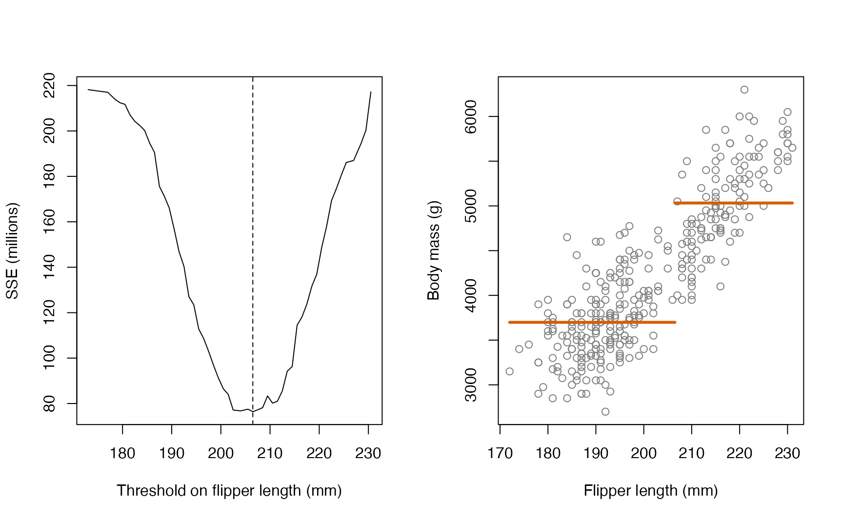
The best split, at 206.5 mm, reduces the SSE by 65% compared with predicting the overall mean. A full regression tree repeats this inside each half, producing a step function with more and more steps.
4. Growing and pruning a tree with rpart
A deliberately large tree
set.seed(2026)
tree_full <- rpart(
  survived ~ ., data = titanic_train, method = "class",
  control = rpart.control(cp = 0, minsplit = 10, xval = 10)
)
nrow(tree_full$frame[tree_full$frame$var == "<leaf>", ])   # number of leaves
#> [1] 50With cp = 0 and minsplit = 10, the tree keeps splitting as long as a node has at least 10 passengers: it grows 50 leaves and certainly overfits. (rpart handles the missing ages itself, using surrogate splits on correlated variables.)
Cost-complexity pruning
Instead of stopping early, the standard strategy is to grow a large tree and then prune it back. For a value \(\alpha \ge 0\), pruning finds the subtree \(T\) that minimises
\[ R_\alpha(T) = R(T) + \alpha\, |T|, \]
where \(R(T)\) is the training error and \(|T|\) the number of leaves. \(\alpha = 0\) keeps the full tree; a large \(\alpha\) prunes everything back to the root. rpart calls a rescaled version of \(\alpha\) the complexity parameter cp, and for every candidate cp it reports a 10-fold cross-validated error:
printcp(tree_full)#>
#> Classification tree:
#> rpart(formula = survived ~ ., data = titanic_train, method = "class",
#> control = rpart.control(cp = 0, minsplit = 10, xval = 10))
#>
#> Variables actually used in tree construction:
#> [1] age embarked fare parch pclass sex sibsp
#>
#> Root node error: 375/981 = 0.38
#>
#> n= 981
#>
#> CP nsplit rel error xerror xstd
#> 1 0.42400 0 1.00 1.00 0.041
#> 2 0.02267 1 0.58 0.58 0.035
#> 3 0.02133 3 0.53 0.55 0.034
#> 4 0.01422 5 0.49 0.53 0.033
#> 5 0.00800 8 0.45 0.51 0.033
#> 6 0.00533 10 0.43 0.52 0.033
#> 7 0.00400 12 0.42 0.54 0.034
#> 8 0.00311 23 0.37 0.52 0.033
#> 9 0.00267 29 0.35 0.53 0.034
#> 10 0.00178 35 0.33 0.53 0.034
#> 11 0.00133 38 0.33 0.53 0.034
#> 12 0.00089 42 0.32 0.56 0.034
#> 13 0.00067 45 0.32 0.57 0.034
#> 14 0.00000 49 0.32 0.57 0.034
TipHow to read this output
- Each row is a subtree.
CPis the complexity parameter at which it becomes optimal,nsplitits number of splits (leaves =nsplit + 1). rel erroris the training error relative to the root (it always decreases).xerroris the cross-validated error relative to the root, andxstdits standard error. These are the columns to use for choosing the size.
plotcp(tree_full)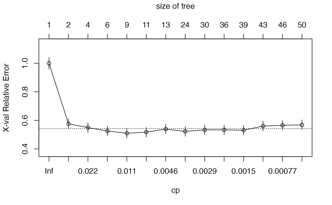
The 1-SE rule — done correctly
Picking the row with the smallest xerror tends to select trees that are larger than necessary: the CV curve is often flat near its minimum, and the exact minimum is partly noise. The one-standard-error rule (Breiman et al., 1984) chooses the simplest tree whose CV error is within one standard error of the minimum:
cpt <- tree_full$cptable
i_min <- which.min(cpt[, "xerror"])                       # minimum CV error
threshold <- cpt[i_min, "xerror"] + cpt[i_min, "xstd"]   # min + 1 SE
i_1se <- which(cpt[, "xerror"] <= threshold)[1]           # simplest such tree
c(splits_min = cpt[i_min, "nsplit"], splits_1se = cpt[i_1se, "nsplit"])
#> splits_min splits_1se
#> 8 5tree_1se <- prune(tree_full, cp = cpt[i_1se, "CP"])Rows of cptable are ordered from the simplest tree (largest cp) to the most complex, so the first row under the threshold is the simplest acceptable tree. (The old version of this lesson announced the 1-SE rule but took which.min(xerror), i.e. the minimum — a different rule.) Here the minimum-error tree has 8 splits and the 1-SE tree 5.
Reading the pruned tree
rpart.plot(tree_1se, extra = 104, under = TRUE)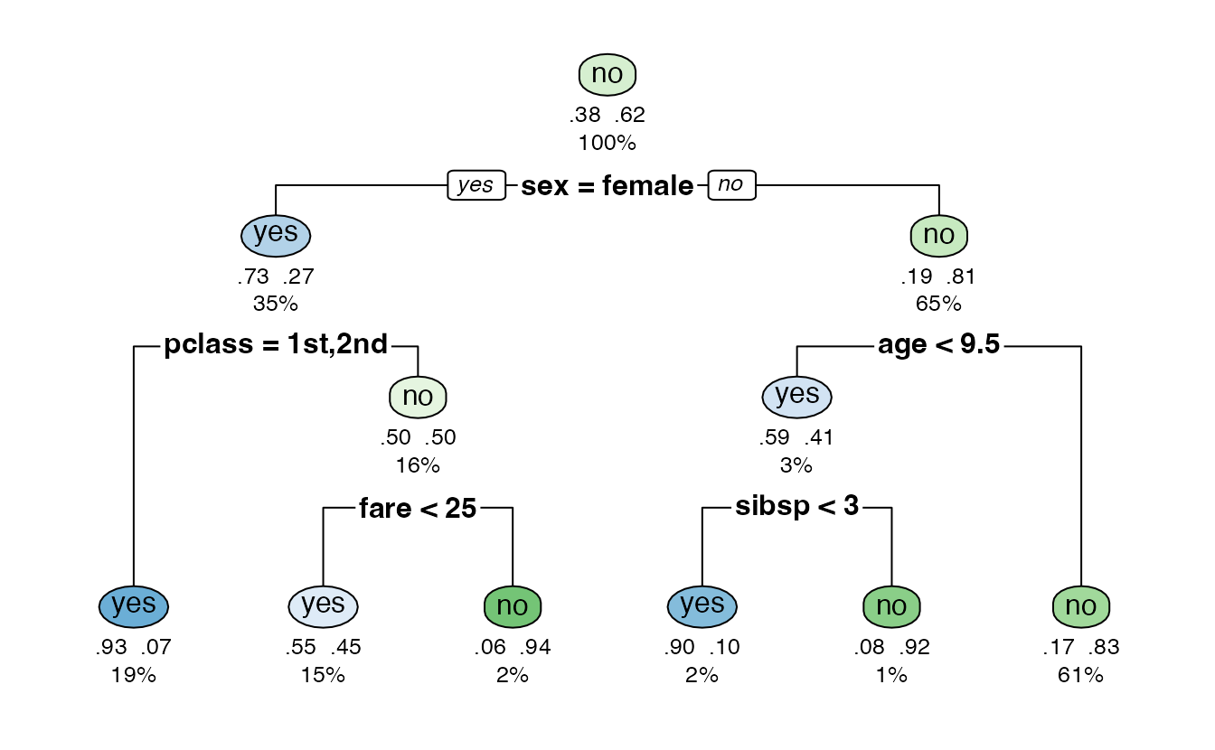
Read a path from the root to a leaf as a rule. The first split is on sex, as our hand calculation suggested. The same rules in text form:
rpart.rules(tree_1se, cover = TRUE)#> survived cover
#> 0.07 when sex is female & pclass is 1st or 2nd 19%
#> 0.10 when sex is male & age < 9.5 & sibsp < 3 2%
#> 0.45 when sex is female & pclass is 3rd & fare < 25 15%
#> 0.83 when sex is male & age >= 9.5 61%
#> 0.92 when sex is male & age < 9.5 & sibsp >= 3 1%
#> 0.94 when sex is female & pclass is 3rd & fare >= 25 2%For a two-class outcome, rpart.rules() prints the fitted probability of the second level of the outcome (here no, i.e. death) — check the column header it prints. cover is the percentage of training passengers following each rule.
5. Tuning a tree with tidymodels
The rpart CV is convenient but specific to rpart. In tidymodels we tune the tree like any other model, with the same folds and metrics as the logistic regression of lesson 44, so the results are directly comparable.
tree_spec <- decision_tree(cost_complexity = tune(), tree_depth = tune(),
                           min_n = 10) |>
  set_engine("rpart") |>
  set_mode("classification")

tree_rec <- recipe(survived ~ ., data = titanic_train) |>
  step_impute_median(all_numeric_predictors()) |>
  step_impute_mode(all_nominal_predictors())

tree_wf <- workflow() |>
  add_recipe(tree_rec) |>
  add_model(tree_spec)
Trees need neither dummy variables nor normalisation, so the recipe only imputes missing values (rpart could also handle them on its own; imputing keeps the pipeline identical across models).
tree_grid <- grid_regular(cost_complexity(),
                          tree_depth(range = c(1L, 10L)),
                          levels = c(5, 4))
nrow(tree_grid)
#> [1] 20set.seed(2026)
tree_res <- tune_grid(tree_wf, resamples = titanic_folds,
grid = tree_grid, metrics = titanic_metrics)A grid of 20 combinations × 5 folds = 100 fits; trees are fast, so this takes seconds.
autoplot(tree_res, metric = c("roc_auc", "brier_class"))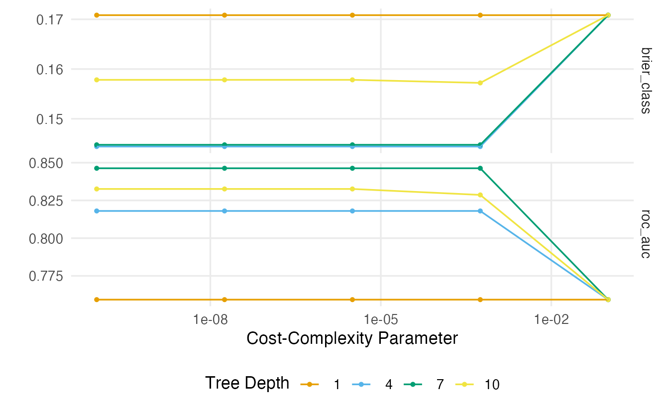
show_best(tree_res, metric = "roc_auc", n = 5)#> # A tibble: 5 × 8
#> cost_complexity tree_depth .metric .estimator mean n std_err .config
#> <dbl> <int> <chr> <chr> <dbl> <int> <dbl> <chr>
#> 1 0.0000000001 7 roc_auc binary 0.8463 5 0.01823 pre0_mod03…
#> 2 0.00000001778 7 roc_auc binary 0.8463 5 0.01823 pre0_mod07…
#> 3 0.000003162 7 roc_auc binary 0.8463 5 0.01823 pre0_mod11…
#> 4 0.0005623 7 roc_auc binary 0.8463 5 0.01823 pre0_mod15…
#> 5 0.0000000001 10 roc_auc binary 0.8326 5 0.01600 pre0_mod04…best_tree <- select_by_one_std_err(tree_res, desc(cost_complexity),
tree_depth, metric = "roc_auc")
best_tree#> # A tibble: 1 × 3
#> cost_complexity tree_depth .config
#> <dbl> <int> <chr>
#> 1 0.0005623 7 pre0_mod15_post0select_best() would return the combination with the highest mean AUC. select_by_one_std_err() implements the 1-SE rule: among combinations within one standard error of the best, it returns the simplest, where we define “simple” by sorting on desc(cost_complexity) (more pruning) and then tree_depth (shallower).
tree_final <- tree_wf |>
  finalize_workflow(best_tree) |>
  last_fit(titanic_split, metrics = titanic_metrics)
collect_metrics(tree_final)
#> # A tibble: 6 × 4
#> .metric .estimator .estimate .config
#> <chr> <chr> <dbl> <chr>
#> 1 accuracy binary 0.8110 pre0_mod0_post0
#> 2 sensitivity binary 0.72 pre0_mod0_post0
#> 3 specificity binary 0.8670 pre0_mod0_post0
#> 4 roc_auc binary 0.8611 pre0_mod0_post0
#> 5 brier_class binary 0.1354 pre0_mod0_post0
#> 6 mn_log_loss binary 0.5359 pre0_mod0_post0tree_final |>
extract_workflow() |>
extract_fit_engine() |>
rpart.plot(extra = 104, under = TRUE)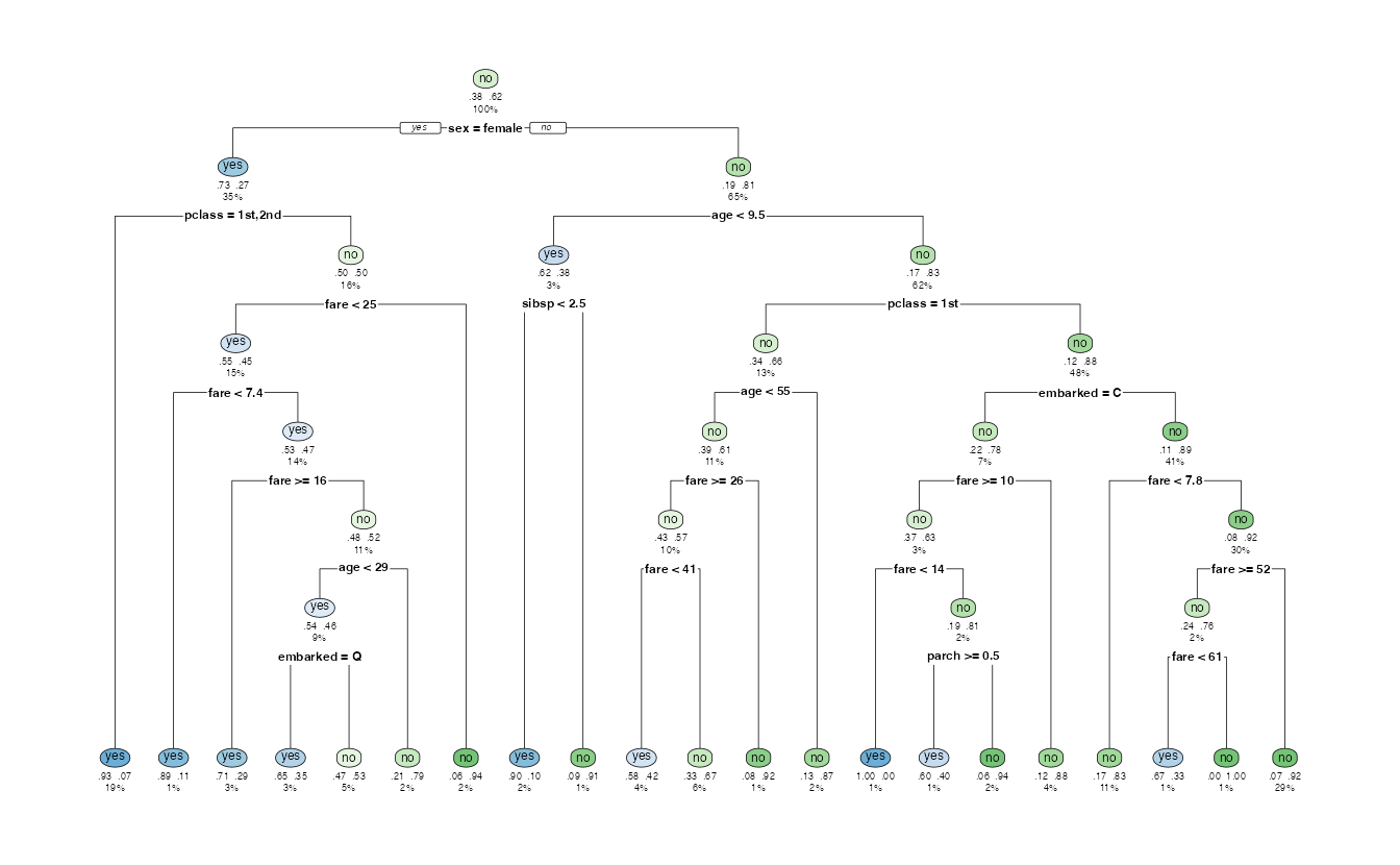
extract_fit_engine() returns the underlying rpart object, so every rpart tool (rpart.plot(), rpart.rules(), printcp()) works on it.
6. Trees are unstable
Fit the same kind of tree on four bootstrap samples of the training data (samples of the same size, drawn with replacement — see the bootstrap lesson):
set.seed(45)
boot_trees <- lapply(1:4, \(b) {
  idx <- sample(nrow(titanic_train), replace = TRUE)
  rpart(survived ~ ., data = titanic_train[idx, ], method = "class",
        control = rpart.control(cp = 0.01))
})
par(mfrow = c(2, 2))
for (tr in boot_trees) rpart.plot(tr, extra = 0, cex = 0.7)
par(mfrow = c(1, 1))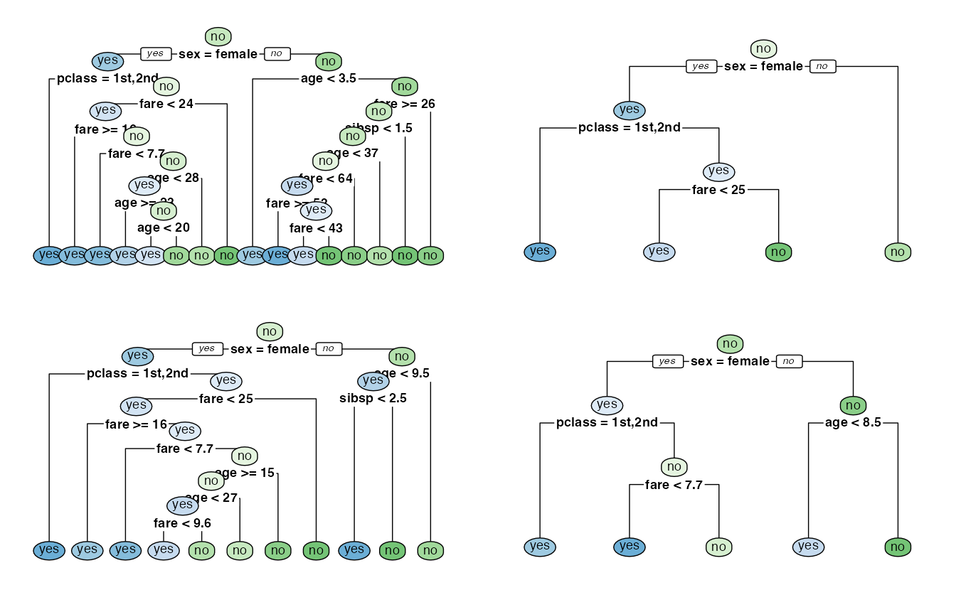
The first split (sex) is stable, because its signal is strong. Below it, the trees choose different variables and thresholds. Predictions for a single passenger can change a lot:
passenger <- tibble(
  pclass = factor("2nd", levels = levels(titanic$pclass)),
  sex = factor("male", levels = levels(titanic$sex)),
  age = 30, sibsp = 0, parch = 0, fare = 13,
  embarked = factor("S", levels = levels(titanic$embarked))
)
set.seed(45)
p_boot <- replicate(50, {
  idx <- sample(nrow(titanic_train), replace = TRUE)
  fit <- rpart(survived ~ ., data = titanic_train[idx, ], method = "class",
               control = rpart.control(cp = 0.01))
  predict(fit, passenger, type = "prob")[, "yes"]
})
summary(p_boot)
#> Min. 1st Qu. Median Mean 3rd Qu. Max.
#> 0.0937 0.1346 0.1593 0.1534 0.1729 0.1969Across 50 bootstrap trees, the predicted survival probability of a 30-year-old man in 2nd class ranges from 0.09 to 0.2. This is the high variance of section 3 of lesson 44, in action. Because each split depends on the previous ones, a small change near the top propagates down the whole tree.
The natural cure is to average many trees: averaging reduces variance. This is the idea behind random forests and, in a different way, boosting.
WarningCommon pitfalls
- Keeping the unpruned tree. A tree grown until leaves are pure has near-zero training error and poor test performance. Prune (or tune
cost_complexity/tree_depth/min_n). - Calling the minimum-xerror tree “the 1-SE tree”. The 1-SE rule picks the simplest tree within one SE of the minimum.
- Over-interpreting the structure. A different sample could give a different tree; interpret only the strong, stable splits.
- Reading
printcp()’srel erroras test error. It is training error; usexerror. - Forgetting
set.seed()beforerpart(): its internal cross-validation is random, soxerrorchanges from run to run.
7. Check your understanding
8. Exercises
★ Exercise 1 — impurity by hand. Using gini() and entropy(), compute the impurity decrease of the split “1st class vs the rest” on titanic. Is it better or worse than the split on sex?
TipSolution
tab_1st <- table(titanic$pclass == "1st", titanic$survived)
w_1st <- rowSums(tab_1st) / sum(tab_1st)
gini(root) - sum(w_1st * apply(tab_1st, 1, gini))
entropy(root) - sum(w_1st * apply(tab_1st, 1, entropy))
The decrease (about 0.04 for Gini) is much smaller than for sex (about 0.13): sex is the better first question.
★★ Exercise 2 — predict the output. Without running it: if you multiply flipper_len by 10 (millimetres → tenths of a millimetre) and rerun best_split(), what happens to the threshold and to the minimum SSE? Then check.
TipSolution
The threshold is multiplied by 10 (it becomes 2065) and the minimum SSE is unchanged: the same penguins end up on each side, so the two group means are the same.
sp10 <- best_split(10 * peng$flipper_len, peng$body_mass)
c(sp10$cut, min(sp10$sse) - min(sp$sse))
★★ Exercise 3 — debug the 1-SE rule. A student writes cp_1se <- cpt[which.min(cpt[, "xerror"] + cpt[, "xstd"]), "CP"]. Explain what this selects, and why it is not the 1-SE rule.
TipSolution
It picks the tree with the smallest value of xerror + xstd — a penalised minimum, which is usually the same tree as (or close to) the minimum-error tree. The 1-SE rule instead computes one threshold (the minimum xerror plus its xstd) and then takes the simplest tree (first row) whose xerror is below that threshold:
i_min <- which.min(cpt[, "xerror"])
i_1se <- which(cpt[, "xerror"] <= cpt[i_min, "xerror"] + cpt[i_min, "xstd"])[1]
★★ Exercise 4 — a regression tree. Fit rpart(body_mass ~ ., data = penguins, method = "anova") (exclude year first). Plot it with rpart.plot(). Which variable is used for the first split? Is it the one you found with best_split() on flipper length alone?
TipSolution
peng_tree <- rpart(body_mass ~ ., method = "anova",
                   data = select(penguins, -year))
rpart.plot(peng_tree)
Because the tree can now choose among all predictors (including species and sex), the first split need not be on flipper length: the algorithm takes the single split with the largest SSE reduction across all variables. Compare the root split in the plot with the threshold 206.5 mm found above. Leaves show the mean body mass (in grams) and the percentage of penguins.
★★★ Exercise 5 — quantify instability. Repeat the bootstrap experiment of section 6 with 100 trees. For each tree record the set of variables it uses (hint: tr$frame$var lists the split variable of every node, and "<leaf>" for leaves). Tabulate the results: how many different variable sets appear?
TipSolution
set.seed(45)
var_sets <- replicate(100, {
  idx <- sample(nrow(titanic_train), replace = TRUE)
  tr <- rpart(survived ~ ., data = titanic_train[idx, ], method = "class",
              control = rpart.control(cp = 0.01))
  used <- setdiff(as.character(tr$frame$var), "<leaf>")
  paste(sort(unique(used)), collapse = ", ")
})
sort(table(var_sets), decreasing = TRUE)
length(unique(var_sets))
sex appears in every tree, but the other variables used (age, pclass, fare, sibsp, …) change from one bootstrap sample to the next, giving many distinct variable sets. Trees that look equally good on the data can tell different stories.
Summary
| Idea / function | What it does |
|---|---|
| Gini \(1-\sum p_k^2\), entropy \(-\sum p_k\log_2 p_k\) | Impurity of a node (classification) |
| SSE around the mean | Impurity of a node (regression) |
rpart(y ~ ., method = "class") |
Grow a tree ("anova" for regression) |
printcp(), plotcp(), prune() |
Cost-complexity path and pruning |
| 1-SE rule | Simplest tree within 1 SE of the minimum CV error |
rpart.plot(), rpart.rules() |
Plot / list the rules |
decision_tree(cost_complexity, tree_depth, min_n) |
tidymodels specification (set_engine("rpart")) |
select_by_one_std_err() |
1-SE rule for any tuning result |
- Trees split the data greedily with the question that most reduces impurity.
- Big trees overfit; pruning trades a little bias for much less variance.
- Trees are easy to read but unstable — small data changes, different trees.
- Averaging many trees fixes the instability: next lesson.