Logistic regression

Modelling yes/no outcomes: odds ratios, predicted probabilities and honest classification

Move from probabilities to odds to log-odds, fit logistic regression with glm(), interpret coefficients as odds ratios, compare models with deviance, and evaluate a classifier with a confusion matrix, ROC/AUC, a threshold chosen on validation data and a calibration plot.

Level 4 · Models & learning ⏱ ~120 min Prerequisites: Multiple regression, Model selection, Proportions and χ²

Learning objectives

By the end of this lesson you will be able to:

convert between probabilities, odds and log-odds and explain why logistic regression uses the log-odds;
fit a logistic regression with glm(family = binomial) and interpret coefficients as odds ratios with confidence intervals;
report predicted probabilities for typical profiles, and compare models with deviance, likelihood-ratio tests and AIC;
evaluate a classifier with a confusion matrix, sensitivity, specificity, precision, ROC/AUC and a calibration plot, choosing the threshold on validation data;
recognise separation and use diagnostics that suit binary outcomes (binned residuals).

library(dplyr)
library(ggplot2)
library(forcats)
library(readr)
library(broom)
library(rsample)
library(yardstick)

1. Why not just use `lm()`?

Many outcomes are binary: a patient recovers or not, a customer buys or not, a penguin is male or female. Code the outcome as 1 (“event”) and 0, and the mean of $y$ for a group of similar units is the probability of the event. So we want to model a probability.

Take Adelie penguins and try to predict sex from body mass and bill depth with an ordinary linear model:

adelie <- penguins |>
  filter(species == "Adelie", !is.na(sex)) |>
  mutate(mass_100g = body_mass / 100)   # body mass in units of 100 g

m_lpm <- lm(as.numeric(sex == "male") ~ mass_100g + bill_dep, data = adelie)
range(fitted(m_lpm))

#> [1] -0.256  1.331

Some “probabilities” are negative and some exceed 1. A straight line has no reason to stay between 0 and 1. We need a model whose predictions are always valid probabilities: logistic regression.

2. Probabilities, odds and log-odds

The odds of an event are the probability that it happens divided by the probability that it does not: $\text{odds} = p / (1 - p)$. Bookmakers use them: odds of 4 (“4 to 1”) mean the event is four times as likely to happen as not, i.e. $p = 0.8$. The log-odds (or logit) is the natural logarithm of the odds.

tibble::tibble(
  probability = c(0.01, 0.1, 0.2, 0.5, 0.8, 0.9, 0.99),
  odds = probability / (1 - probability),
  log_odds = log(odds)          # same as qlogis(probability)
)

#> # A tibble: 7 × 3
#>   probability     odds log_odds
#>         <dbl>    <dbl>    <dbl>
#> 1        0.01  0.01010   -4.595
#> 2        0.1   0.1111    -2.197
#> 3        0.2   0.25      -1.386
#> 4        0.5   1          0    
#> 5        0.8   4          1.386
#> 6        0.9   9          2.197
#> 7        0.99 99.00       4.595

Notice the three scales:

probability lives between 0 and 1;
odds live between 0 and $+\infty$, with 1 meaning “50–50”;
log-odds live on the whole real line, are 0 at $p = 0.5$, and are symmetric: $p = 0.2$ and $p = 0.8$ give $-1.39$ and $+1.39$.

Because the log-odds can take any value, we can model them with a linear predictor $\beta_0 + \beta_1 x_1 + \dots$ without ever producing an impossible probability. Converting back gives the logistic curve:

\[ \log\frac{p}{1-p} = \beta_0 + \beta_1 x \quad\Longleftrightarrow\quad p = \frac{1}{1 + e^{-(\beta_0 + \beta_1 x)}} . \]

tibble::tibble(log_odds = seq(-6, 6, by = 0.1),
               probability = plogis(log_odds)) |>
  ggplot(aes(log_odds, probability)) +
  geom_line(linewidth = 1) +
  geom_hline(yintercept = c(0, 1), linetype = 3) +
  labs(x = "Log-odds (linear predictor)", y = "Probability")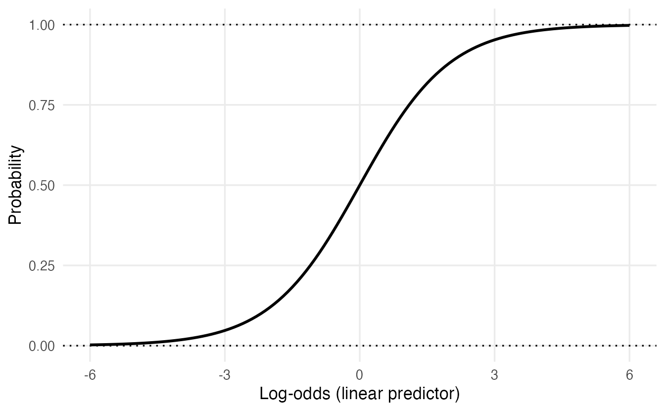

Figure 1: The logistic curve maps any log-odds value (x axis) to a probability between 0 and 1. It is steepest at p = 0.5.

In R, plogis() converts log-odds to probabilities and qlogis() does the reverse.

3. Fitting a logistic regression with `glm()`

Logistic regression is a generalized linear model (GLM): a linear predictor, a link function (here the logit) connecting it to the mean, and a distribution for $y$ (here Bernoulli/binomial). glm() fits it by maximum likelihood (it finds the coefficients that make the observed 0s and 1s most probable).

m_sex <- glm(sex ~ mass_100g + bill_dep, family = binomial, data = adelie)
summary(m_sex)

#> 
#> Call:
#> glm(formula = sex ~ mass_100g + bill_dep, family = binomial, 
#>     data = adelie)
#> 
#> Coefficients:
#>             Estimate Std. Error z value Pr(>|z|)    
#> (Intercept)  -45.977      8.452   -5.44  5.3e-08 ***
#> mass_100g      0.718      0.145    4.96  7.1e-07 ***
#> bill_dep       1.065      0.342    3.12   0.0018 ** 
#> ---
#> Signif. codes:  0 '***' 0.001 '**' 0.01 '*' 0.05 '.' 0.1 ' ' 1
#> 
#> (Dispersion parameter for binomial family taken to be 1)
#> 
#>     Null deviance: 202.399  on 145  degrees of freedom
#> Residual deviance:  76.151  on 143  degrees of freedom
#> AIC: 82.15
#> 
#> Number of Fisher Scoring iterations: 7

When the response is a factor, glm() models the probability of the second level. levels(adelie$sex) is c("female", "male"), so we are modelling $P(\text{male})$. Check this every time — it determines the sign of every coefficient.

How to read this output

Coefficients are on the log-odds scale. Holding bill depth constant, each extra 100 g of body mass increases the log-odds of being male by 0.72. Positive = higher probability of “male”.
z value and Pr(>|z|) — Wald tests of $H_0: \beta = 0$ (estimate / SE, compared to a normal distribution, hence z, not t).
Dispersion parameter … taken to be 1 — for binary data the variance is fixed by the mean: $p(1-p)$. There is no separate $\sigma$.
Null deviance / Residual deviance — how badly the intercept-only model and our model fit (lower = better; see Section 6).
AIC — as in Model selection.
Fisher Scoring iterations — the number of steps of the fitting algorithm. Very large numbers (≥ 25) can signal separation (Section 10).

4. Interpretation: odds ratios

Log-odds are hard to think in. Exponentiating a coefficient gives an odds ratio (OR): the factor by which the odds are multiplied when the predictor increases by one unit, holding the others constant.

exp(coef(m_sex))

#> (Intercept)   mass_100g    bill_dep 
#>   1.077e-20   2.051e+00   2.902e+00

exp(confint(m_sex))    # profile-likelihood 95% CIs, then exponentiated

#>                 2.5 %    97.5 %
#> (Intercept) 5.865e-29 2.174e-14
#> mass_100g   1.599e+00 2.839e+00
#> bill_dep    1.564e+00 6.071e+00

Body mass: for each extra 100 g, the odds of being male are multiplied by 2.05 (95% CI 1.6 to 2.84), for penguins with the same bill depth.
Bill depth: each extra mm multiplies the odds by 2.9, holding mass constant.
An OR of 1 means no association; OR > 1 increases the odds, OR < 1 decreases them. A CI for the OR that excludes 1 corresponds to p < 0.05.

The same with broom (exponentiate = TRUE transforms both estimates and CIs):

tidy(m_sex, exponentiate = TRUE, conf.int = TRUE)

#> # A tibble: 3 × 7
#>   term         estimate std.error statistic       p.value  conf.low conf.high
#>   <chr>           <dbl>     <dbl>     <dbl>         <dbl>     <dbl>     <dbl>
#> 1 (Intercept) 1.077e-20    8.452     -5.440 0.00000005332 5.865e-29 2.174e-14
#> 2 mass_100g   2.051e+ 0    0.1448     4.960 0.0000007060  1.599e+ 0 2.839e+ 0
#> 3 bill_dep    2.902e+ 0    0.3419     3.116 0.001832      1.564e+ 0 6.071e+ 0

Ignore the intercept’s OR: it is the odds for a penguin with 0 g mass and 0 mm bill depth.

Odds ratios are not risk ratios

“OR = 2” means the odds double, not the probability. If $p = 0.5$ (odds 1), doubling the odds gives odds 2, i.e. $p = 0.67$; if $p = 0.9$ (odds 9), doubling gives odds 18, i.e. $p = 0.95$. The change in probability depends on where you start. That is why we also report predicted probabilities.

5. Predicted probabilities

predict(..., type = "response") returns probabilities; the default type = "link" returns log-odds. A good way to communicate a model is to predict for a few typical profiles:

profiles <- tibble::tibble(mass_100g = c(32, 37, 42),
                           bill_dep = mean(adelie$bill_dep))
profiles |>
  mutate(p_male = predict(m_sex, newdata = profiles, type = "response"))

#> # A tibble: 3 × 3
#>   mass_100g bill_dep  p_male
#>       <dbl>    <dbl>   <dbl>
#> 1        32    18.35 0.03101
#> 2        37    18.35 0.5374 
#> 3        42    18.35 0.9768

An Adelie of average bill depth weighing 3200 g is very likely female; at 3700 g it is a coin toss; at 4200 g it is very likely male.

For confidence intervals, compute them on the link scale (where the normal approximation is good) and transform the limits:

grid <- tibble::tibble(mass_100g = seq(28, 48, by = 0.25),
                       bill_dep = mean(adelie$bill_dep))
link <- predict(m_sex, newdata = grid, type = "link", se.fit = TRUE)
grid <- grid |>
  mutate(p = plogis(link$fit),
         lower = plogis(link$fit - 1.96 * link$se.fit),
         upper = plogis(link$fit + 1.96 * link$se.fit))

ggplot(grid, aes(100 * mass_100g, p)) +
  geom_ribbon(aes(ymin = lower, ymax = upper), alpha = 0.25) +
  geom_line(linewidth = 1) +
  geom_jitter(data = adelie, aes(body_mass, as.numeric(sex == "male")),
              height = 0.03, width = 0, alpha = 0.4) +
  labs(x = "Body mass (g)", y = "P(male)")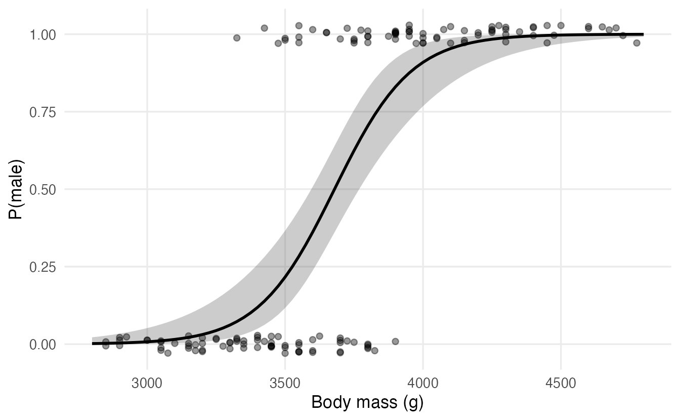

Figure 2: Predicted probability of being male for Adelie penguins of average bill depth, with a 95% confidence band. Dots: observed sex (0 = female, 1 = male).

Average marginal effects

Another summary on the probability scale is the average marginal effect (AME): the average, over all penguins in the data, of the change in predicted probability for a small increase in a predictor. For logistic regression the derivative of $p$ with respect to $x_j$ is $\beta_j\,p(1-p)$, so:

p_hat <- fitted(m_sex)
mean(coef(m_sex)["mass_100g"] * p_hat * (1 - p_hat))

#> [1] 0.05811

On average, 100 g more body mass raises the probability of being male by about 6 percentage points (for small changes). The marginaleffects package computes AMEs, with standard errors, for any model:

marginaleffects::avg_slopes(m_sex, variables = "mass_100g")

6. Deviance, likelihood-ratio tests and AIC

The deviance generalises the residual sum of squares: it measures how far the fitted model is from a perfect fit (lower = better). The difference in deviance between two nested models follows, approximately, a $\chi^2$ distribution with degrees of freedom equal to the number of added parameters: this is the likelihood-ratio test (LRT).

m0 <- glm(sex ~ 1, family = binomial, data = adelie)
m1 <- glm(sex ~ mass_100g, family = binomial, data = adelie)
anova(m0, m1, m_sex, test = "Chisq")

#> Analysis of Deviance Table
#> 
#> Model 1: sex ~ 1
#> Model 2: sex ~ mass_100g
#> Model 3: sex ~ mass_100g + bill_dep
#>   Resid. Df Resid. Dev Df Deviance Pr(>Chi)    
#> 1       145      202.4                         
#> 2       144       88.7  1    113.7  < 2e-16 ***
#> 3       143       76.2  1     12.6  0.00039 ***
#> ---
#> Signif. codes:  0 '***' 0.001 '**' 0.01 '*' 0.05 '.' 0.1 ' ' 1

AIC(m0, m1, m_sex)

#>       df    AIC
#> m0     1 204.40
#> m1     2  92.74
#> m_sex  3  82.15

How to read this output

Resid. Dev falls from 202.4 (intercept only) to 88.7 with body mass, and to 76.2 with bill depth added.
Each row tests the model against the one above: body mass reduces the deviance by 113.7 on 1 df; adding bill depth reduces it further by 12.6 (p = 0.00039). Both terms improve the fit.
AIC agrees: the two-predictor model has the lowest value.

The LRT is generally more reliable than the Wald z-test in the summary table, especially in small samples. (test = "LRT" is a synonym for "Chisq".)

Going deeper: likelihood and deviance

For binary $y_i$ with fitted probabilities $\hat p_i$, the log-likelihood is

\[ \ell = \sum_i \big[y_i \log \hat p_i + (1 - y_i)\log(1 - \hat p_i)\big], \]

and for 0/1 data the deviance is $D = -2\ell$ (the saturated model has likelihood 1). The LRT statistic for nested models is $D_0 - D_1 \sim \chi^2_{p_1 - p_0}$ under $H_0$. There is no closed-form solution for $\hat\beta$; glm() uses iteratively reweighted least squares, a sequence of weighted linear regressions.

7. From probabilities to classes: the confusion matrix

To classify, we choose a threshold $t$ and predict “male” when $\hat p > t$. With $t = 0.5$:

pred_class <- if_else(fitted(m_sex) > 0.5, "male", "female")
cm <- table(predicted = pred_class, observed = adelie$sex)
cm

#>          observed
#> predicted female male
#>    female     67    9
#>    male        6   64

Call “male” the positive class (the event). Then:

	observed positive	observed negative
predicted positive	true positive (TP)	false positive (FP)
predicted negative	false negative (FN)	true negative (TN)

tp <- cm["male", "male"];   fn <- cm["female", "male"]
tn <- cm["female", "female"]; fp <- cm["male", "female"]
c(accuracy    = (tp + tn) / sum(cm),
  sensitivity = tp / (tp + fn),   # recall: share of males found
  specificity = tn / (tn + fp),   # share of females correctly identified
  precision   = tp / (tp + fp))   # share of "male" predictions that are right

#>    accuracy sensitivity specificity   precision 
#>      0.8973      0.8767      0.9178      0.9143

These values are computed on the same data used to fit the model, so they are optimistic. For an honest evaluation we need new data — which brings us to a larger example.

8. A real example: predicting income

The adult.csv file contains 48,842 records from the 1994 US Census. The goal: predict whether a person earns more than 50,000 dollars a year.

Import and clean

adult_raw <- read_csv(data_path("adult.csv"), na = c("", "?"),
                      show_col_types = FALSE)
glimpse(adult_raw)

#> Rows: 48,842
#> Columns: 10
#> $ x                 <dbl> 1, 2, 3, 4, 5, 6, 7, 8, 9, 10, 11, 12, 13, 14, 15, 1…
#> $ age               <dbl> 25, 38, 28, 44, 18, 34, 29, 63, 24, 55, 65, 36, 26, …
#> $ workclass         <chr> "Private", "Private", "Local-gov", "Private", NA, "P…
#> $ education         <chr> "11th", "HS-grad", "Assoc-acdm", "Some-college", "So…
#> $ `educational-num` <dbl> 7, 9, 12, 10, 10, 6, 9, 15, 10, 4, 9, 13, 9, 9, 9, 1…
#> $ `marital-status`  <chr> "Never-married", "Married-civ-spouse", "Married-civ-…
#> $ race              <chr> "Black", "White", "White", "Black", "White", "White"…
#> $ gender            <chr> "Male", "Male", "Male", "Male", "Female", "Male", "M…
#> $ `hours-per-week`  <dbl> 40, 50, 40, 40, 30, 30, 40, 32, 40, 10, 40, 40, 39, …
#> $ income            <chr> "<=50K", "<=50K", ">50K", ">50K", "<=50K", "<=50K", …

The file codes missing values as "?", and the column names contain hyphens. We clean the categories with forcats:

adult <- adult_raw |>
  select(-x) |>                                    # row index
  rename_with(\(nm) gsub("-", "_", nm)) |>         # marital-status -> marital_status
  mutate(
    income = factor(income, levels = c("<=50K", ">50K"),
                    labels = c("low", "high")),
    workclass = factor(workclass) |>
      fct_na_value_to_level(level = "Unknown") |>  # NA becomes a level
      fct_lump_min(min = 100, other_level = "Other"),
    education = fct_collapse(
      education,
      "No HS diploma" = c("Preschool", "1st-4th", "5th-6th", "7th-8th",
                          "9th", "10th", "11th", "12th"),
      "HS grad"       = "HS-grad",
      "Some college"  = c("Some-college", "Assoc-acdm", "Assoc-voc"),
      "Bachelors"     = "Bachelors",
      "Postgraduate"  = c("Masters", "Prof-school", "Doctorate")
    ) |>
      fct_relevel("No HS diploma", "HS grad", "Some college", "Bachelors"),
    marital = fct_collapse(
      marital_status,
      "Married"       = c("Married-civ-spouse", "Married-AF-spouse"),
      "Never married" = "Never-married",
      other_level     = "Other"
    ) |>
      fct_relevel("Married", "Never married"),
    race = fct_infreq(race),                       # most frequent = reference
    gender = factor(gender),
    age_10 = age / 10,                             # age in decades
    hours_10 = hours_per_week / 10                 # hours in units of 10
  ) |>
  select(income, age_10, hours_10, education, marital, gender, race,
         workclass)

count(adult, income) |> mutate(prop = n / sum(n))

#> # A tibble: 2 × 3
#>   income     n   prop
#>   <fct>  <int>  <dbl>
#> 1 low    37155 0.7607
#> 2 high   11687 0.2393

A few decisions worth explaining:

fct_na_value_to_level(): about 6% of workclass is missing. Dropping those rows would waste data (and they may not be missing at random); a separate “Unknown” level keeps them and lets the model estimate their own effect.
fct_lump_min(): “Without-pay” and “Never-worked” have only 21 and 10 people — far too few to estimate a coefficient. Lumping rare levels into “Other” stabilises the model.
fct_collapse(): 16 education levels become 5 interpretable groups. We drop educational_num, which is just a numeric code for education: including both would put the same information in the model twice.
Rescaling by fixed constants (age / 10) is harmless: it uses no information from the data. Standardising (subtracting the mean, dividing by the SD) would use the data; it is not needed for glm(), and if it were needed it would have to be estimated on the training set only.
About 24% of people are in the “high” class: the outcome is imbalanced.

Split: training, validation and test

We need three sets: training to fit the model, validation to choose the classification threshold, and test to evaluate the final choice once. Stratifying by income keeps the class proportions the same in all three.

set.seed(2026)
adult_split <- initial_validation_split(adult, prop = c(0.6, 0.2),
                                        strata = income)
adult_train <- training(adult_split)
adult_val   <- validation(adult_split)
adult_test  <- testing(adult_split)
c(train = nrow(adult_train), validation = nrow(adult_val),
  test = nrow(adult_test))

#>      train validation       test 
#>      29305       9768       9769

Fit and interpret

m_inc <- glm(income ~ age_10 + hours_10 + education + marital + gender +
               race + workclass,
             family = binomial, data = adult_train)

tidy(m_inc, exponentiate = TRUE, conf.int = TRUE) |>
  filter(term != "(Intercept)") |>
  select(term, odds_ratio = estimate, conf.low, conf.high) |>
  mutate(across(where(is.numeric), \(x) round(x, 2)))

#> # A tibble: 20 × 4
#>    term                      odds_ratio conf.low conf.high
#>    <chr>                          <dbl>    <dbl>     <dbl>
#>  1 age_10                          1.33     1.29      1.37
#>  2 hours_10                        1.34     1.3       1.38
#>  3 educationHS grad                2.94     2.52      3.44
#>  4 educationSome college           5.28     4.53      6.18
#>  5 educationBachelors             14.21    12.12     16.73
#>  6 educationPostgraduate          30.43    25.51     36.41
#>  7 maritalNever married            0.08     0.07      0.09
#>  8 maritalOther                    0.12     0.1       0.13
#>  9 genderMale                      1.14     1.03      1.25
#> 10 raceBlack                       0.76     0.66      0.87
#> 11 raceAsian-Pac-Islander          0.85     0.7       1.03
#> 12 raceAmer-Indian-Eskimo          0.72     0.48      1.04
#> 13 raceOther                       0.69     0.43      1.08
#> 14 workclassLocal-gov              0.54     0.44      0.67
#> 15 workclassPrivate                0.62     0.51      0.74
#> 16 workclassSelf-emp-inc           0.9      0.71      1.14
#> 17 workclassSelf-emp-not-inc       0.37     0.3       0.46
#> 18 workclassState-gov              0.5      0.4       0.64
#> 19 workclassUnknown                0.26     0.2       0.34
#> 20 workclassOther                  0.13     0.01      0.78

Reading a few odds ratios (all “holding the other predictors constant”):

Education: compared with people without a high-school diploma, the odds of high income are about 14 times higher for those with a bachelor’s degree, and about 30 times higher with a postgraduate degree.
Marital status: never-married people have odds about 0.08 times those of married people — roughly 13 times lower.
Hours: each additional 10 weekly hours multiplies the odds by 1.34.
Gender: the adjusted OR for men is only 1.14. The raw difference between men and women is much larger, but in these data much of it overlaps with the other predictors, above all marital status, which is strongly associated with both gender and high income — a reminder that adjusted coefficients depend on what else is in the model, and are not causal effects.

Diagnostics: binned residuals

The residual plots of lm() are useless here: with a 0/1 outcome, residuals fall on two curves whatever the model. Instead, bin the observations (e.g. by a predictor or by the fitted probability) and look at the average residual $y - \hat p$ in each bin. If the model is right, the averages should be close to 0, mostly inside $\pm 2$ standard errors.

binned_resid <- function(model, data, by) {
  data |>
    mutate(p = fitted(model), r = as.numeric(income == "high") - p,
           bin = ntile({{ by }}, 20)) |>
    summarise(x = mean({{ by }}), mean_resid = mean(r),
              se = sqrt(sum(p * (1 - p))) / n(), .by = bin)
}

binned_resid(m_inc, adult_train, age_10) |>
  ggplot(aes(10 * x, mean_resid)) +
  geom_hline(yintercept = 0) +
  geom_line(aes(y = 2 * se), linetype = 2) +
  geom_line(aes(y = -2 * se), linetype = 2) +
  geom_point() +
  labs(x = "Age (years, bin average)", y = "Average residual")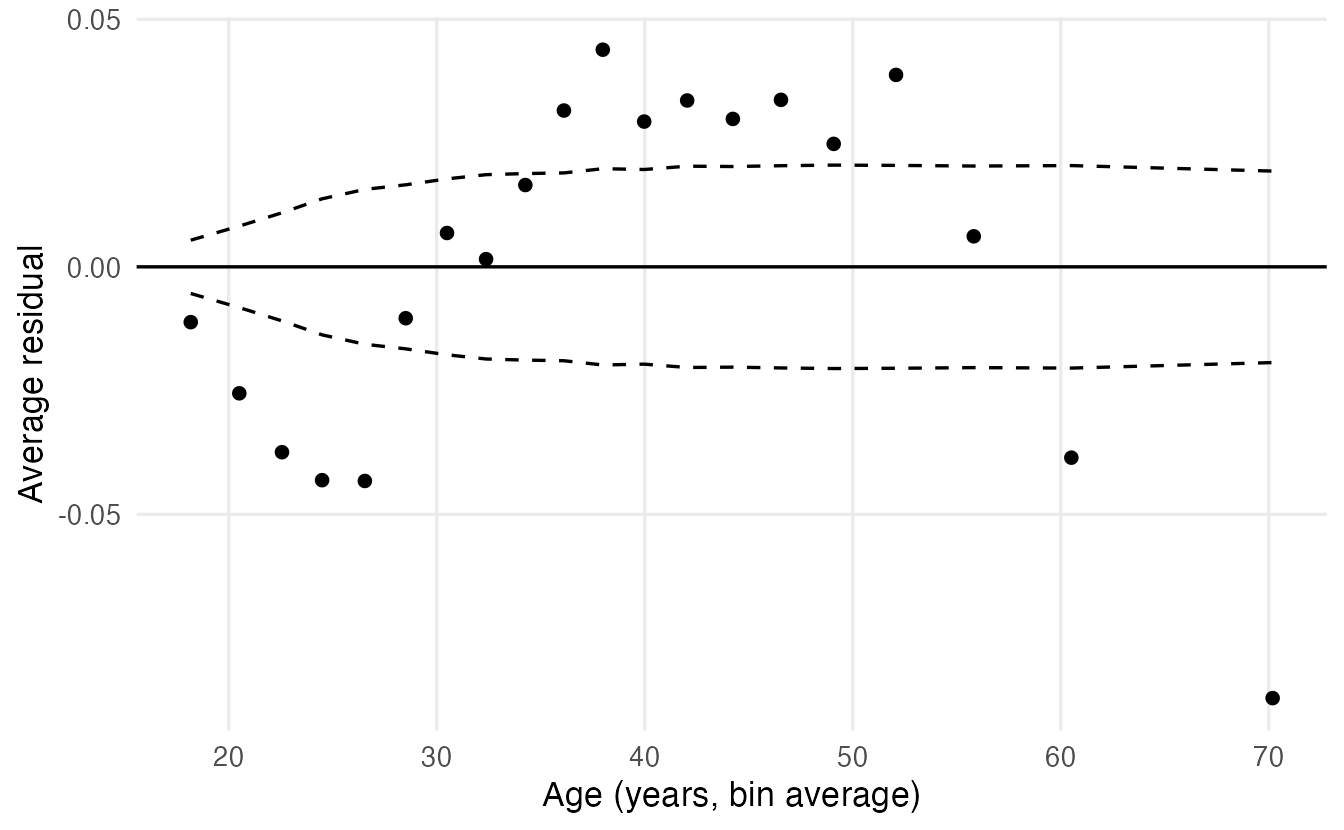

Figure 3: Binned residuals against age (training data). The inverted-U pattern shows that a straight line in age is not enough.

The model under-predicts high income in middle age and over-predicts it for the young and the old: income rises with age and then falls. A quadratic term captures this:

m_inc2 <- update(m_inc, . ~ . + I(age_10^2))
anova(m_inc, m_inc2, test = "Chisq")

#> Analysis of Deviance Table
#> 
#> Model 1: income ~ age_10 + hours_10 + education + marital + gender + race + 
#>     workclass
#> Model 2: income ~ age_10 + hours_10 + education + marital + gender + race + 
#>     workclass + I(age_10^2)
#>   Resid. Df Resid. Dev Df Deviance Pr(>Chi)    
#> 1     29284      21445                         
#> 2     29283      21063  1      382   <2e-16 ***
#> ---
#> Signif. codes:  0 '***' 0.001 '**' 0.01 '*' 0.05 '.' 0.1 ' ' 1

AIC(m_inc, m_inc2)

#>        df   AIC
#> m_inc  21 21487
#> m_inc2 22 21107

The deviance drops by 382 for a single extra parameter. Re-draw the binned residual plot with m_inc2 (Exercise 3): the pattern disappears. With a quadratic term, the OR of age_10 alone is no longer interpretable; show the effect of age with predicted probabilities across ages instead.

9. Evaluating the classifier honestly

Accuracy can mislead

A “model” that predicts “low” for everyone is right about 76% of the time on the validation set — without learning anything. With imbalanced classes, accuracy mostly rewards predicting the majority class. Always look at sensitivity and specificity (or precision), and at threshold-free measures such as AUC.

Predictions on the validation set

val_pred <- adult_val |>
  mutate(.pred_high = predict(m_inc2, newdata = adult_val,
                              type = "response"))

ROC curve and AUC

Each threshold gives a pair (sensitivity, specificity). The ROC curve plots sensitivity against 1 − specificity for all thresholds; the AUC (area under the curve) is the probability that a randomly chosen “high” person gets a higher predicted probability than a randomly chosen “low” person (0.5 = coin toss, 1 = perfect ranking).

In yardstick, the event is the first factor level by default. Our levels are c("low", "high"), so we must say event_level = "second":

roc_auc(val_pred, truth = income, .pred_high, event_level = "second")

#> # A tibble: 1 × 3
#>   .metric .estimator .estimate
#>   <chr>   <chr>          <dbl>
#> 1 roc_auc binary        0.8810

roc_curve(val_pred, truth = income, .pred_high, event_level = "second") |>
  ggplot(aes(1 - specificity, sensitivity)) +
  geom_path(linewidth = 1) +
  geom_abline(linetype = 2) +
  coord_equal() +
  labs(x = "1 - specificity (false positive rate)",
       y = "Sensitivity (true positive rate)")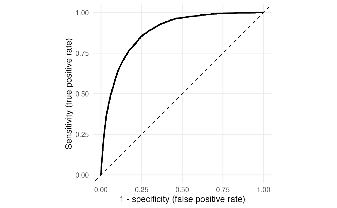

Figure 4: ROC curve of the income model on the validation set. The dashed diagonal is a model that guesses at random.

Forgetting event_level = "second" would silently report $1 - \text{AUC}$ and a mirrored curve.

Choosing the threshold on the validation set

The default threshold of 0.5 is rarely the right one. With 24% positives, it finds only about half of the high earners. Which threshold is “best” depends on the costs of the two errors; a neutral choice is to maximise Youden’s J = sensitivity + specificity − 1. We compute it on the validation set for a grid of thresholds:

class_summary <- function(prob, is_event, t) {
  pred <- prob > t
  c(threshold   = t,
    sensitivity = sum(pred & is_event) / sum(is_event),
    specificity = sum(!pred & !is_event) / sum(!is_event),
    precision   = sum(pred & is_event) / sum(pred))
}

thresholds <- seq(0.05, 0.95, by = 0.01)
grid_t <- lapply(thresholds, \(t) class_summary(
  val_pred$.pred_high, val_pred$income == "high", t)) |>
  bind_rows() |>
  mutate(youden = sensitivity + specificity - 1)

best_t <- grid_t$threshold[which.max(grid_t$youden)]
best_t

#> [1] 0.23

grid_t |>
  tidyr::pivot_longer(c(sensitivity, specificity, precision),
                      names_to = "metric") |>
  ggplot(aes(threshold, value, colour = metric)) +
  geom_line(linewidth = 1) +
  geom_vline(xintercept = best_t, linetype = 3) +
  labs(x = "Threshold", y = NULL, colour = NULL)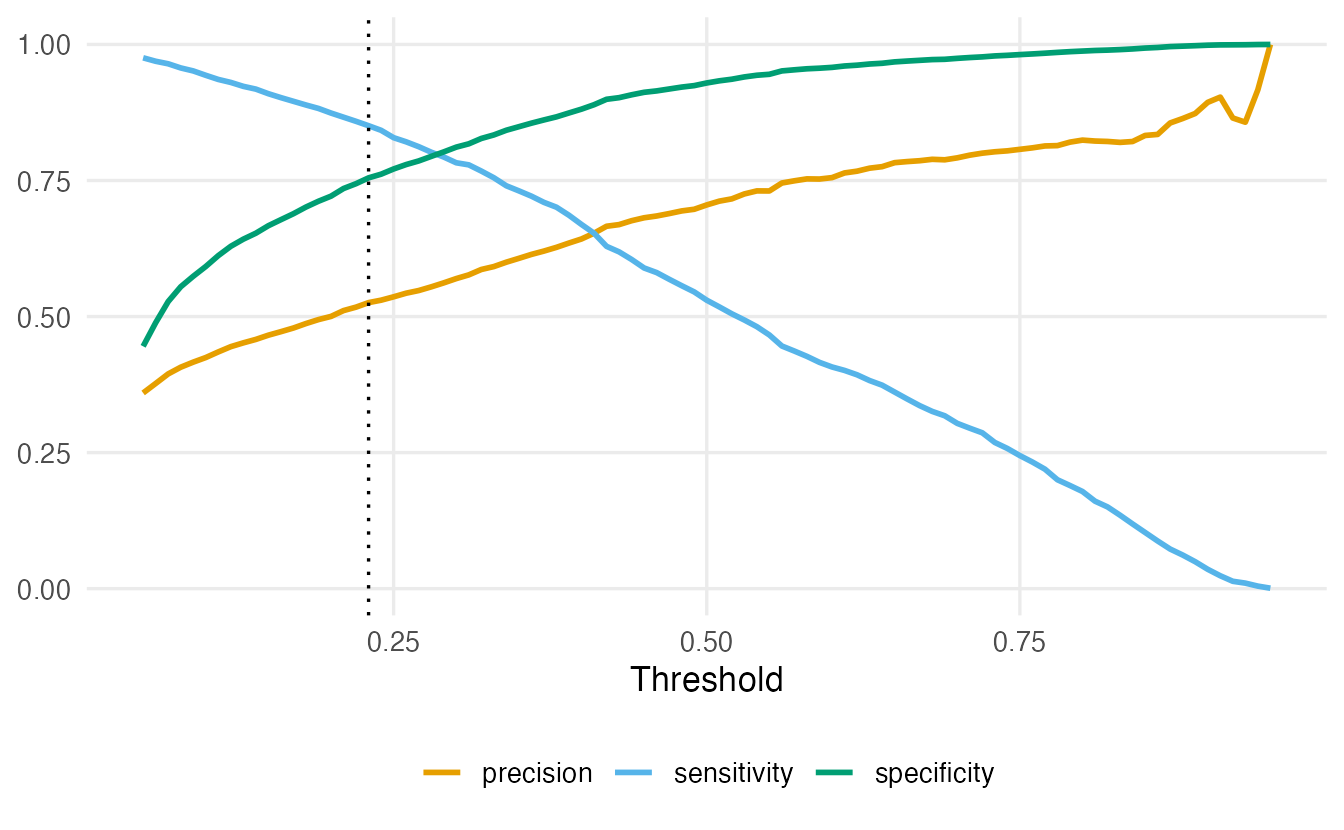

Figure 5: Sensitivity, specificity and precision on the validation set as the threshold varies. The dotted line marks the threshold that maximises Youden’s J.

Raising the threshold makes the model more conservative: fewer false positives (specificity and precision up), more missed positives (sensitivity down). If missing a positive is costly (e.g. a disease), choose a lower threshold; if false alarms are costly, a higher one. The choice belongs to the validation set, not to the test set.

Final evaluation on the test set — once

test_pred <- adult_test |>
  mutate(
    .pred_high = predict(m_inc2, newdata = adult_test, type = "response"),
    .pred_class = factor(if_else(.pred_high > best_t, "high", "low"),
                         levels = levels(income))
  )

conf_mat(test_pred, truth = income, estimate = .pred_class)

#>           Truth
#> Prediction  low high
#>       low  5612  351
#>       high 1846 1960

class_metrics <- metric_set(accuracy, sens, spec, precision)
class_metrics(test_pred, truth = income, estimate = .pred_class,
              event_level = "second")

#> # A tibble: 4 × 3
#>   .metric   .estimator .estimate
#>   <chr>     <chr>          <dbl>
#> 1 accuracy  binary        0.7751
#> 2 sens      binary        0.8481
#> 3 spec      binary        0.7525
#> 4 precision binary        0.5150

roc_auc(test_pred, truth = income, .pred_high, event_level = "second")

#> # A tibble: 1 × 3
#>   .metric .estimator .estimate
#>   <chr>   <chr>          <dbl>
#> 1 roc_auc binary        0.8824

How to read this output

conf_mat() shows predictions in rows and the truth in columns.
With the threshold chosen on validation data, the model finds most high earners (sensitivity) at the price of more false alarms (lower precision) than at 0.5.
The test AUC is close to the validation AUC: no sign that we overfitted the validation set.
These test numbers are our honest estimate of performance on new people from the same population.

Calibration: are the probabilities right?

A model can rank people well (high AUC) and still give wrong probabilities. A calibration plot groups test observations into bins of predicted probability and compares the average prediction with the observed proportion of events:

test_pred |>
  mutate(bin = ntile(.pred_high, 10)) |>
  summarise(predicted = mean(.pred_high),
            observed = mean(income == "high"),
            n = n(), .by = bin) |>
  ggplot(aes(predicted, observed)) +
  geom_abline(linetype = 2) +
  geom_line() +
  geom_point(size = 2) +
  coord_equal(xlim = c(0, 1), ylim = c(0, 1)) +
  labs(x = "Mean predicted probability", y = "Observed proportion high")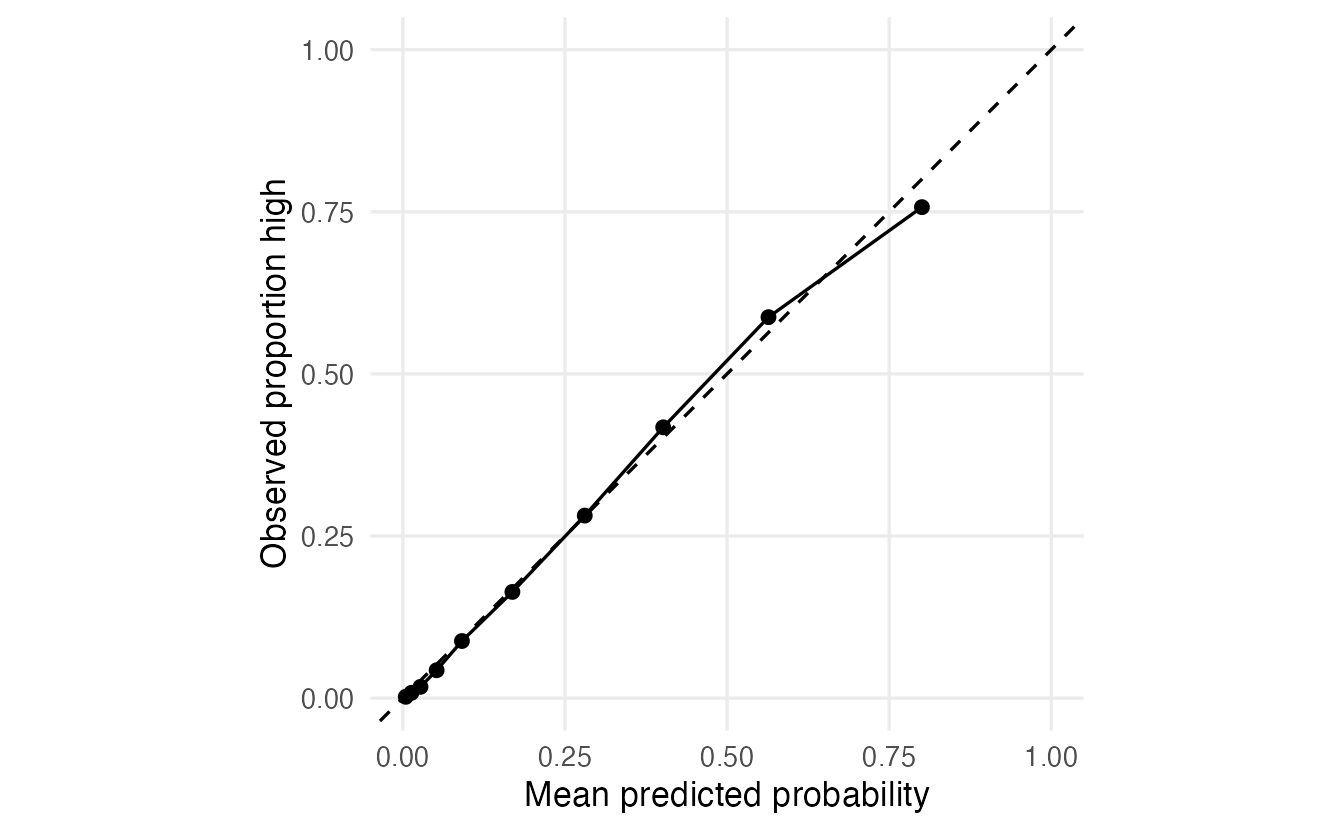

Figure 6: Calibration plot on the test set (10 bins of predicted probability). Points near the diagonal mean that predicted probabilities match observed frequencies.

Logistic regression fitted by maximum likelihood is usually well calibrated on data like the training data; more flexible machine learning models often are not (see Model comparison).

10. Separation: when coefficients run away

Can we tell Adelie from Gentoo penguins by bill depth and flipper length?

two_species <- penguins |>
  filter(species %in% c("Adelie", "Gentoo")) |>
  droplevels()

m_sep <- glm(species ~ bill_dep + flipper_len, family = binomial,
             data = two_species)

R warns that the algorithm did not converge and that fitted probabilities numerically 0 or 1 occurred. summary(m_sep) shows enormous coefficients and standard errors. This is (complete) separation: a combination of the predictors classifies every bird perfectly, so the maximum likelihood estimate is infinite — the curve wants to become a vertical step.

Separation is not a bug in your code. It means the predictors determine the outcome in this sample. Options: report that the groups are perfectly separable (sometimes that is the finding), drop or merge the offending categories, or use penalised estimators such as Firth’s logistic regression (package logistf) or a ridge/lasso penalty (Penalized regression), which give finite, shrunken estimates.

Common pitfalls

Not checking which level is the event. glm() models the second factor level; yardstick treats the first as the event unless you set event_level = "second". Mixing them up flips signs or AUCs silently.
Reading coefficients as changes in probability. They are changes in log-odds; exponentiate for odds ratios, and use predicted probabilities or AMEs for the probability scale.
Calling an odds ratio a “risk” ratio. When the event is common, the two differ a lot.
Choosing the threshold on the test set — or hard-coding one “chosen on validation” without computing it. Compute it on validation data; use the test set once.
Judging a classifier by accuracy with imbalanced classes. Look at sensitivity, specificity, precision, AUC and calibration.
Preprocessing before splitting. Scaling, imputing or selecting with all the data leaks information from the test set. Fixed transformations (like age / 10) are fine; anything estimated from data belongs in the training step (with recipes from lesson 44).
Using plot(glm_model) diagnostics designed for lm(). Use binned residuals and calibration plots instead.

11. Check your understanding

Q1. A coefficient on the log-odds scale is −0.69. What is the odds ratio, and what does it mean?

$e^{-0.69} \approx 0.50$: each one-unit increase in the predictor halves the odds of the event, holding the other predictors constant.

Q2. The probability of an event is 0.75. What are the odds and the log-odds?

Odds = 0.75 / 0.25 = 3 (“3 to 1”); log-odds = log(3) ≈ 1.10.

Q3. A classifier has AUC = 0.88 but its predicted probabilities are all between 0.4 and 0.6. Is that a problem?

It ranks people well (AUC), but it is badly calibrated: the probabilities cannot be taken at face value (an event rate of 5% or 95% in some groups is reported as about 50%). Check a calibration plot before using probabilities for decisions.

Q4. Why do we need a validation set in addition to the test set here?

Because we make a data-driven choice (the threshold). If we chose it on the test set, the test performance would be optimistic. The validation set absorbs the choice; the test set stays untouched for the final, honest estimate. (Cross-validation on the training set is an alternative to a separate validation set.)

12. Exercises

★ Exercise 1 — odds ratios. Using adelie, fit glm(sex ~ bill_len, family = binomial). Report the odds ratio per mm of bill length with its 95% CI and write one sentence interpreting it.

Solution

m_bl <- glm(sex ~ bill_len, family = binomial, data = adelie)
tidy(m_bl, exponentiate = TRUE, conf.int = TRUE)

The OR is about 2.0 per mm (95% CI roughly 1.6 to 2.5): each additional millimetre of bill length roughly doubles the odds of being male. Remember that the model describes $P(\text{male})$ because “male” is the second level.

★★ Exercise 2 — predict the output. Without running it: what is exp(confint(m_sex))["mass_100g", ] if body mass is entered in grams (body_mass) instead of hundreds of grams? Then check.

Solution

The coefficient per gram is 1/100 of the coefficient per 100 g, so the OR per gram is the 100th root of the OR per 100 g: about $2.05^{1/100} \approx 1.007$, with CI about 1.005 to 1.010. The model and its predictions are identical; only the unit changes. Choose units that make the OR readable.

m_g <- glm(sex ~ body_mass + bill_dep, family = binomial, data = adelie)
exp(confint(m_g))["body_mass", ]

★★ Exercise 3 — diagnostics. Draw the binned residual plot for m_inc2 (with the quadratic age term) using binned_resid(). Then draw a second binned residual plot against hours_10 for m_inc2. Is the linear effect of hours adequate?

Solution

plot_binned <- function(df, xlab) {
  ggplot(df, aes(x, mean_resid)) +
    geom_hline(yintercept = 0) +
    geom_line(aes(y = 2 * se), linetype = 2) +
    geom_line(aes(y = -2 * se), linetype = 2) +
    geom_point() +
    labs(x = xlab, y = "Average residual")
}
binned_resid(m_inc2, adult_train, age_10) |> plot_binned("Age (decades)")
binned_resid(m_inc2, adult_train, hours_10) |> plot_binned("Hours / 10")

Against age, the inverted U is gone. Against hours, the residuals show a pattern too: many people work exactly 40 hours, and the effect of hours is not linear (it flattens beyond about 50 hours). A quadratic term or a spline for hours would improve the model — try adding I(hours_10^2) and compare AIC.

★★ Exercise 4 — debug. A student computes the AUC and gets 0.12:

val_pred |> roc_auc(truth = income, .pred_high)

What went wrong? What about roc_auc(val_pred, truth = income, 1 - .pred_high)?

Solution

yardstick treats the first level ("low") as the event, but .pred_high is the probability of the second level. The result is $1 - \text{AUC}$. Fix it with event_level = "second". The second version is also correct, because $1 - \hat p$ is the predicted probability of “low”, the first level — but it is less readable. Being explicit with event_level is the safer habit.

★★★ Exercise 5 — mini-analysis: a different threshold rule. Suppose that missing a high earner costs three times as much as a false alarm (e.g. a bank marketing a premium product). On the validation set, find the threshold that minimises total cost $3 \times \text{FN} + 1 \times \text{FP}$. Compare it with best_t, then report sensitivity and precision on the test set at the new threshold.

Solution

cost <- sapply(thresholds, \(t) {
  pred <- val_pred$.pred_high > t
  truth <- val_pred$income == "high"
  3 * sum(!pred & truth) + sum(pred & !truth)
})
t_cost <- thresholds[which.min(cost)]
t_cost

class_summary(test_pred$.pred_high, test_pred$income == "high", t_cost)

The cost-based threshold is close to $1/(1 + 3) = 0.25$ — the theoretical optimum for a well-calibrated model with these costs — and in the same region as best_t. On the test set sensitivity is high (around 0.85) and precision moderate (around 0.5). A different cost ratio would give a different threshold: the “best” threshold is a decision, not a property of the model.

Summary

Idea / function	What it does
`qlogis(p)`, `plogis(x)`	probability → log-odds, log-odds → probability
`glm(y ~ x, family = binomial)`	logistic regression (models the second level)
`exp(coef(m))`, `exp(confint(m))`	odds ratios and their CIs
`tidy(m, exponentiate = TRUE, conf.int = TRUE)`	odds-ratio table
`predict(m, newdata, type = "response")`	predicted probabilities
`anova(m0, m1, test = "Chisq")`, `AIC()`	likelihood-ratio test, model comparison
`initial_validation_split(strata = )`	train / validation / test split
`roc_auc()`, `roc_curve()` with `event_level = "second"`	AUC and ROC curve
`conf_mat()`, `metric_set(accuracy, sens, spec, precision)`	confusion matrix and class metrics
binned residuals, calibration plot	diagnostics for binary outcomes

Logistic regression is linear on the log-odds scale; exponentiated coefficients are odds ratios.
Communicate with predicted probabilities for meaningful profiles, not only with ORs.
Classification needs a threshold, chosen on validation data according to the costs of errors.
With imbalanced classes, accuracy misleads: report sensitivity, specificity, precision, AUC — and check calibration.
Warnings about fitted probabilities of 0 or 1 signal separation: the MLE does not exist.

1. Why not just use lm()?

2. Probabilities, odds and log-odds

3. Fitting a logistic regression with glm()

4. Interpretation: odds ratios

5. Predicted probabilities

Average marginal effects

6. Deviance, likelihood-ratio tests and AIC

7. From probabilities to classes: the confusion matrix

8. A real example: predicting income

Import and clean

Split: training, validation and test

Fit and interpret

Diagnostics: binned residuals

9. Evaluating the classifier honestly

Accuracy can mislead

Predictions on the validation set

ROC curve and AUC

Choosing the threshold on the validation set

Final evaluation on the test set — once

Calibration: are the probabilities right?

10. Separation: when coefficients run away

11. Check your understanding

12. Exercises

Summary

1. Why not just use `lm()`?

3. Fitting a logistic regression with `glm()`