Recurrent networks and LSTM for time series

Forecasting hourly electricity demand from its recent past — and checking against simple baselines

Frame forecasting as supervised learning with sliding windows, split a time series in time order, understand recurrent networks, vanishing gradients and LSTM gates, and compare an LSTM with naive, seasonal-naive and linear autoregressive forecasts.

Level 4 · Models & learning ⏱ ~90 min Prerequisites: DNNs for tabular data, Multiple regression

NoteLearning objectives

By the end of this lesson you will be able to:

• turn a time series into a supervised dataset of sliding windows and split it in time order;
• compute and interpret naive, seasonal-naive and linear autoregressive baseline forecasts;
• explain how a recurrent network processes a sequence and why plain RNNs suffer from vanishing gradients;
• describe the gates of an LSTM and count its parameters;
• fit an LSTM with layer_lstm() and evaluate it on the original scale with RMSE and MAE.

library(dplyr)
library(tidyr)
library(ggplot2)

library(keras3)

ImportantRunning this lesson

The model chunks need keras3 and a backend (see lesson 61); the data come from the CRAN package tsibbledata (install.packages("tsibbledata")). The results on this page were computed once and frozen. Without keras, the keras code is shown but not run, and numbers that depend on it read “not computed”. All baselines run in plain R.

1. Why forecast demand?

An electricity grid must produce, at every moment, as much power as people consume; storing electricity is expensive. Operators therefore forecast demand hour by hour. The past of the series itself is the main source of information: demand at 6 pm today looks a lot like demand at 5 pm today and at 6 pm yesterday.

The original version of this lesson used an hourly series from a US grid operator downloaded from a third-party website. Here we use a similar, stable source that installs with R: the half-hourly electricity demand of the state of Victoria (Australia), 2012–2014, from the tsibbledata package, aggregated to hours.

2. The data

elec <- tsibbledata::vic_elec |>
  tibble::as_tibble() |>
  arrange(Time) |>
  mutate(hour_id = (row_number() - 1) %/% 2) |>   # pair consecutive half-hours
  summarise(time = first(Time), date = first(Date),
            demand = sum(Demand), temp = mean(Temperature),
            .by = hour_id)
nrow(elec)

#> [1] 26304

range(elec$date)

#> [1] "2012-01-01" "2014-12-31"

Each row is now one hour: demand is the total demand in that hour (MWh) and temp the mean temperature in Melbourne. Always sort a time series by time before doing anything else — the original lesson’s data were not in chronological order, which silently scrambled every window.

p_year <- ggplot(elec, aes(time, demand)) +
  geom_line(linewidth = 0.2, colour = "steelblue") +
  labs(x = NULL, y = "MWh per hour")
p_week <- elec |>
  filter(date >= as.Date("2013-06-03"), date < as.Date("2013-06-17")) |>
  ggplot(aes(time, demand)) +
  geom_line(linewidth = 0.6, colour = "steelblue") +
  labs(x = NULL, y = "MWh per hour")
patchwork::wrap_plots(p_year, p_week, ncol = 1)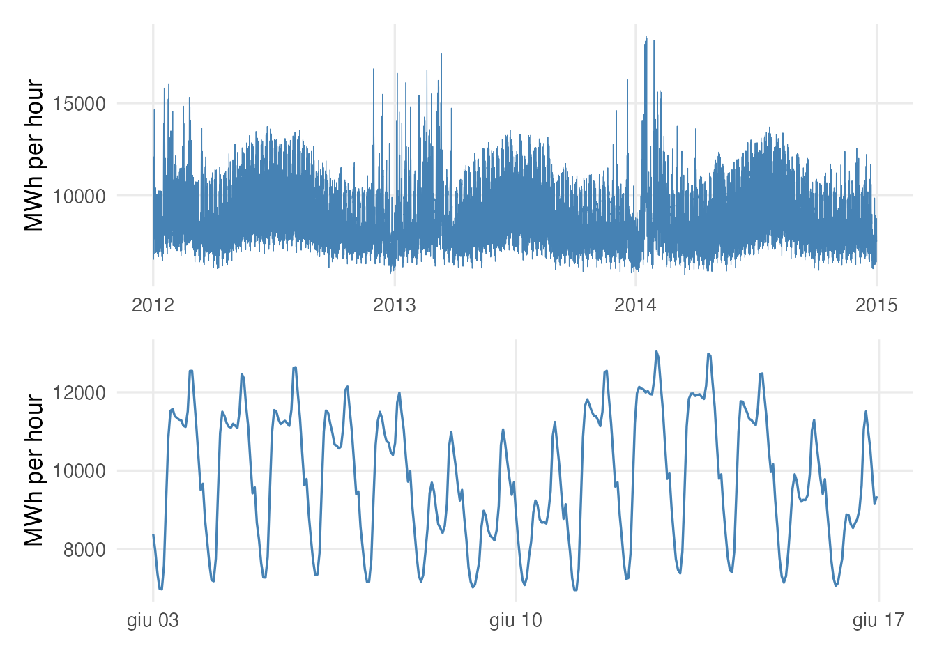

Figure 1: Hourly electricity demand in Victoria. Top: three years (yearly pattern, summer peaks from air conditioning). Bottom: two weeks (daily cycle and weekends).

3. Splitting a time series: always in time order

In earlier lessons we split rows at random. For forecasting that would be cheating: a random test hour would be surrounded by training hours from just before and just after. We must mimic real use — train on the past, evaluate on the future:

• training: 2012–2013,
• validation: January–June 2014 (for early stopping),
• test: July–December 2014 (touched once, at the end).

train_end <- max(which(elec$date <  as.Date("2014-01-01")))
valid_end <- max(which(elec$date <  as.Date("2014-07-01")))
n <- nrow(elec)
c(train = train_end, valid = valid_end - train_end, test = n - valid_end)

#> train valid  test 
#> 17544  4345  4415

We standardise with the mean and standard deviation of the training period only:

mu  <- mean(elec$demand[1:train_end])
sdv <- sd(elec$demand[1:train_end])
z <- (elec$demand - mu) / sdv            # whole series, training scale

4. From a series to a table: sliding windows

A network needs inputs and targets. For one-step-ahead forecasting, each example is a window of the last \(L\) hours (inputs) and the next hour (target):

\[ \text{input } (z_{t-L}, \dots, z_{t-1}) \;\longrightarrow\; \text{target } z_t . \]

Here is the idea on a toy series of 8 values with \(L = 3\):

make_windows <- function(series, target_idx, L) {
  idx <- outer(target_idx, L:1, "-")          # row i: t_i - L, ..., t_i - 1
  X <- matrix(series[idx], nrow = length(target_idx))
  list(X = array(X, dim = c(length(target_idx), L, 1)),   # samples, time, features
       y = series[target_idx])
}
toy <- make_windows(c(10, 11, 12, 13, 14, 15, 16, 17), target_idx = 4:8, L = 3)
toy$X[, , 1]

#>      [,1] [,2] [,3]
#> [1,]   10   11   12
#> [2,]   11   12   13
#> [3,]   12   13   14
#> [4,]   13   14   15
#> [5,]   14   15   16

toy$y

#> [1] 13 14 15 16 17

Each row of the matrix is one example; the corresponding element of y is the value right after it. keras expects recurrent inputs as a 3-D array (samples, time steps, features), hence the last dimension of size 1 (one feature: demand).

We use windows of \(L = 48\) hours. The targets of each set are the hours of that period; their input windows may reach back into the previous period, which is legitimate (those values are already observed when the forecast is made).

L <- 48
w_train <- make_windows(z, (L + 1):train_end, L)
w_valid <- make_windows(z, (train_end + 1):valid_end, L)
w_test  <- make_windows(z, (valid_end + 1):n, L)
dim(w_train$X)

#> [1] 17496    48     1

(The original lesson built the test windows from the training and validation values by mistake, so its “test” score was computed on data the model had already seen. Indexing by target hour, as here, avoids that error.)

5. Baselines: how good is “no model”?

Before any network, three forecasts every analyst should compute:

• naive: next hour = this hour, \(\hat z_t = z_{t-1}\);
• seasonal naive: next hour = same hour yesterday (\(z_{t-24}\)) or last week (\(z_{t-168}\));
• linear autoregression AR(48): a multiple regression of \(z_t\) on the 48 previous values, fitted by lm() on the training windows.

test_idx <- (valid_end + 1):n
lag_df <- function(w) as.data.frame(matrix(w$X, nrow = dim(w$X)[1]))

ar_fit <- lm(y ~ ., data = cbind(y = w_train$y, lag_df(w_train)))
to_mwh <- function(zz) zz * sdv + mu

forecasts <- tibble(
  truth          = elec$demand[test_idx],
  naive          = elec$demand[test_idx - 1],
  seasonal_day   = elec$demand[test_idx - 24],
  seasonal_week  = elec$demand[test_idx - 168],
  ar_48          = to_mwh(predict(ar_fit, newdata = lag_df(w_test)))
)

score <- function(fc) {
  fc |>
    pivot_longer(-truth, names_to = "method", values_to = "forecast") |>
    summarise(rmse = sqrt(mean((truth - forecast)^2)),
              mae  = mean(abs(truth - forecast)), .by = method) |>
    arrange(rmse)
}
score(forecasts)

#> # A tibble: 4 × 3
#>   method         rmse   mae
#>   <chr>         <dbl> <dbl>
#> 1 ar_48         150.5 105.3
#> 2 naive         542.9 415.0
#> 3 seasonal_week 707.8 504.2
#> 4 seasonal_day  972.5 647.4

TipHow to read this output

• RMSE (root mean squared error) and MAE (mean absolute error) are in the units of the data, MWh per hour; lower is better. RMSE penalises large errors more.
• One hour ahead, demand changes slowly, so even the naive forecast is not bad. The seasonal-naive forecasts are worse here because a day (or week) is long enough for weather to change.
• The linear AR(48) model combines all 48 lags with estimated weights and is a demanding benchmark: RMSE 150 versus 543 for the naive forecast.

6. Recurrent networks: reading a sequence step by step

A dense network would treat the 48 input hours as 48 unrelated columns. A recurrent neural network (RNN) instead reads the window in order, one hour at a time, and keeps a hidden state \(h_t\) — a vector that summarises what it has seen so far:

\[ h_t = \tanh\big(W x_t + U h_{t-1} + b\big), \qquad \hat y = v^\top h_L + c . \]

The same weights \(W, U, b\) are used at every time step (just as a CNN reuses a filter across an image, lesson 66), so the number of parameters does not depend on the window length.

Vanishing and exploding gradients

To train an RNN, backpropagation runs through time: the error at the end is sent back step by step. At each step it is multiplied by a factor that depends on \(U\) and on the derivative of the activation. If that factor is typically below 1 the gradient vanishes; above 1 it explodes:

steps <- c(1, 5, 10, 20, 50)
rbind(steps, factor_0.9 = round(0.9^steps, 4), factor_1.1 = round(1.1^steps, 1))

#>            [,1]   [,2]    [,3]    [,4]     [,5]
#> steps       1.0 5.0000 10.0000 20.0000  50.0000
#> factor_0.9  0.9 0.5905  0.3487  0.1216   0.0052
#> factor_1.1  1.1 1.6000  2.6000  6.7000 117.4000

After 50 steps a factor of 0.9 leaves 0.0052 of the signal: information from 50 hours ago has essentially no influence on the weight updates, so a plain RNN cannot learn long-range patterns such as “same hour yesterday”.

7. LSTM: a memory with gates

The Long Short-Term Memory cell (Hochreiter & Schmidhuber, 1997) adds a second state, the cell state \(c_t\), which runs along the sequence like a conveyor belt and is changed only by additions controlled by three gates. Each gate is a layer of sigmoid neurons with values between 0 (closed) and 1 (open):

Gate	Question it answers
Forget gate \(f_t\)	How much of the old memory \(c_{t-1}\) should be kept?
Input gate \(i_t\)	How much of the new candidate information should be written?
Output gate \(o_t\)	How much of the memory should be exposed as the hidden state \(h_t\)?

Because the memory is updated by addition (\(c_t = f_t \odot c_{t-1} + \dots\)) and the forget gate can stay close to 1, the gradient can flow back over many steps without vanishing.

NoteGoing deeper: the LSTM equations and its parameter count

With input \(x_t \in \mathbb R^p\) and \(u\) units,

\[ \begin{aligned} f_t &= \sigma(W_f x_t + U_f h_{t-1} + b_f), & i_t &= \sigma(W_i x_t + U_i h_{t-1} + b_i), \\ o_t &= \sigma(W_o x_t + U_o h_{t-1} + b_o), & \tilde c_t &= \tanh(W_c x_t + U_c h_{t-1} + b_c), \\ c_t &= f_t \odot c_{t-1} + i_t \odot \tilde c_t, & h_t &= o_t \odot \tanh(c_t). \end{aligned} \]

There are four blocks of weights, each with \(u \times p\) input weights, \(u \times u\) recurrent weights and \(u\) biases: \(4\,(u(u+p) + u)\) parameters. With \(u = 32\) and \(p = 1\) that is 4352. Since \(\partial c_t / \partial c_{t-1} = f_t\) (element-wise, ignoring indirect paths), the gradient along the cell state is multiplied by the forget gate rather than by a squashing derivative — the key to its long memory.

8. Fitting an LSTM

The architecture is minimal: one LSTM layer of 32 units reads the 48-hour window; its final hidden state feeds a dense layer with one linear output (a regression, so no activation and mean squared error loss).

set_random_seed(123)
lstm <- keras_model_sequential(input_shape = c(L, 1)) |>
  layer_lstm(units = 32) |>
  layer_dense(units = 1)
lstm |> compile(optimizer = optimizer_adam(learning_rate = 1e-3),
                loss = "mse", metrics = list("mae"))
lstm

#> Model: "sequential"
#> ┏━━━━━━━━━━━━━━━━━━━━━━━━━━━━━━━━━━━┳━━━━━━━━━━━━━━━━━━━━━━━━━━┳━━━━━━━━━━━━━━━┓
#> ┃ Layer (type)                      ┃ Output Shape             ┃       Param # ┃
#> ┡━━━━━━━━━━━━━━━━━━━━━━━━━━━━━━━━━━━╇━━━━━━━━━━━━━━━━━━━━━━━━━━╇━━━━━━━━━━━━━━━┩
#> │ lstm (LSTM)                       │ (None, 32)               │         4,352 │
#> ├───────────────────────────────────┼──────────────────────────┼───────────────┤
#> │ dense (Dense)                     │ (None, 1)                │            33 │
#> └───────────────────────────────────┴──────────────────────────┴───────────────┘
#>  Total params: 4,385 (17.13 KB)
#>  Trainable params: 4,385 (17.13 KB)
#>  Non-trainable params: 0 (0.00 B)

callbacks <- list(
  callback_early_stopping(monitor = "val_loss", patience = 5,
                          restore_best_weights = TRUE),
  callback_reduce_lr_on_plateau(monitor = "val_loss", factor = 0.5,
                                patience = 3)
)
history <- lstm |> fit(
  x = w_train$X, y = w_train$y,
  validation_data = list(w_valid$X, w_valid$y),
  epochs = 30, batch_size = 128,
  callbacks = callbacks, verbose = 0
)

Two callbacks: early stopping as in lesson 62, and callback_reduce_lr_on_plateau(), which halves the learning rate when the validation loss stalls — smaller steps often help in the final phase.

You may wonder whether fit() should shuffle the windows: it does by default, and that is fine. Each window carries its own history, so the order of the examples in training does not matter. What must respect time is the split (Section 3), not the order of mini-batches.

as.data.frame(history) |>
  filter(!is.na(value), metric == "loss") |>
  ggplot(aes(epoch, value, colour = data)) +
  geom_line(linewidth = 0.8) +
  labs(x = "Epoch", y = "MSE (standardised)", colour = NULL)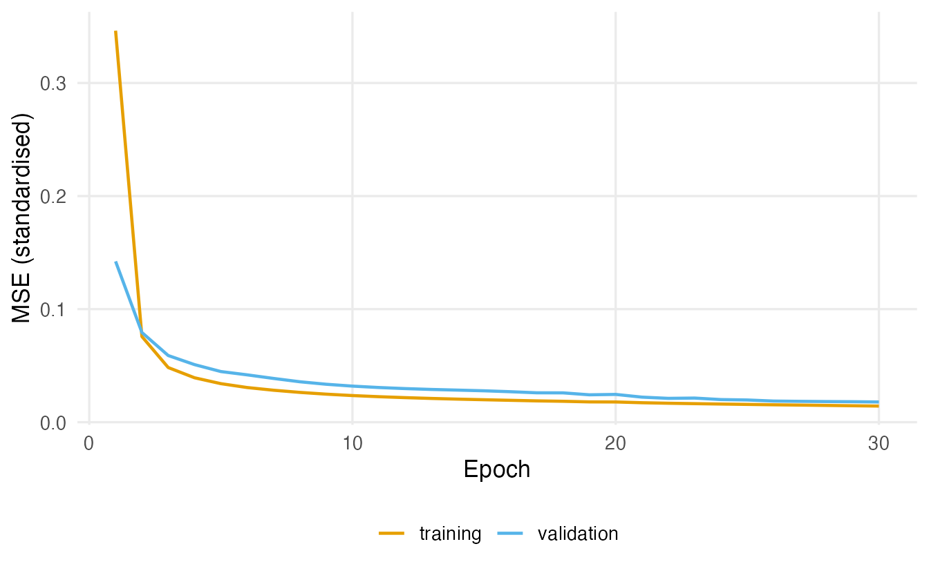

Figure 2: LSTM learning curves (mean squared error on the standardised scale).

9. Evaluation on the test period

forecasts$lstm <- to_mwh(as.vector(predict(lstm, w_test$X, verbose = 0)))
scores <- score(forecasts)
scores

#> # A tibble: 5 × 3
#>   method         rmse   mae
#>   <chr>         <dbl> <dbl>
#> 1 ar_48         150.5 105.3
#> 2 lstm          213.1 158.5
#> 3 naive         542.9 415.0
#> 4 seasonal_week 707.8 504.2
#> 5 seasonal_day  972.5 647.4

TipHow to read this output

The table ranks all methods by test RMSE (MWh per hour, July–December 2014). The LSTM’s RMSE is 213, against 150 for the linear AR(48) and 543 for the naive forecast. The important comparison is with AR(48): it uses exactly the same 48 inputs, and is fitted in a fraction of a second. If the LSTM’s advantage is small, the honest conclusion is that, for one-hour-ahead forecasts of this series, most of the predictable structure is linear.

forecasts |>
  mutate(time = elec$time[test_idx]) |>
  slice_head(n = 168) |>
  select(time, truth, lstm, ar_48) |>
  pivot_longer(-time, names_to = "series", values_to = "mwh") |>
  ggplot(aes(time, mwh, colour = series)) +
  geom_line(linewidth = 0.7) +
  labs(x = NULL, y = "MWh per hour", colour = NULL)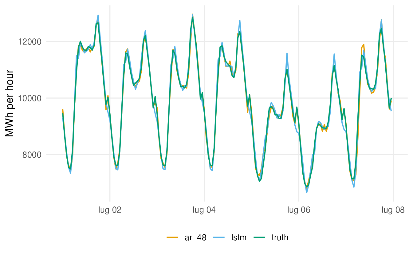

Figure 3: The first week of the test period: observed demand and one-step-ahead forecasts.

WarningCommon pitfalls

1. Random train/test splits for time series. The test period must come after the training period.
2. Scaling with statistics of the whole series. Use the training period only.
3. Unsorted data. Sort by time first; one swapped block corrupts every window that contains it.
4. Building validation or test windows from the wrong segment. Index windows by target time and check that the targets of the test set are exactly the test observations.
5. No baselines. A “good-looking” forecast plot means little if the naive forecast looks just as good. Always report naive, seasonal-naive and a linear model.
6. Reporting errors on the standardised scale only. Transform back to the original units before interpreting RMSE and MAE.

10. Check your understanding

NoteQ1. With windows of length \(L = 48\) and a training series of 17,544 hours, how many training windows are there for one-step-ahead forecasting?

\(17{,}544 - 48 = 17{,}496\): the first 48 hours can only be inputs, never targets.

NoteQ2. Why can a plain RNN not learn that demand at 6 pm depends on demand at 6 pm the day before?

That dependence spans 24 steps. During backpropagation through time, the gradient is multiplied at each step by a factor that is typically less than 1, so after 24 steps it is too small to influence the weights (vanishing gradient).

NoteQ3. What does a forget gate value close to 1 mean?

Keep almost all of the previous cell state: the memory is carried forward unchanged.

11. Exercises

★ Exercise 1 — predict the output. Without running it, write down w$X[, , 1] and w$y for w <- make_windows(c(5, 7, 9, 11, 13), target_idx = 3:5, L = 2). Then check.

TipSolution

Rows are \((z_{t-2}, z_{t-1})\) for \(t = 3, 4, 5\): (5, 7), (7, 9), (9, 11); targets 9, 11, 13.

★ Exercise 2 — count the parameters. How many parameters does layer_lstm(units = 16) have when each time step has 2 features (demand and temperature)? Add the following layer_dense(units = 1).

TipSolution

LSTM: \(4\,(16\cdot(16+2) + 16) = 4 \cdot 304 = 1216\). Dense: \(16 + 1 = 17\). Total 1233.

★★ Exercise 3 — add temperature. Electricity demand depends on temperature (heating in winter, air conditioning in summer). Build windows with two features per time step — standardised demand and standardised temperature — and refit the LSTM with input_shape = c(L, 2). Does the test RMSE improve?

TipSolution

temp_z <- (elec$temp - mean(elec$temp[1:train_end])) / sd(elec$temp[1:train_end])
make_windows2 <- function(target_idx, L) {
  idx <- outer(target_idx, L:1, "-")
  X <- array(c(z[idx], temp_z[idx]), dim = c(length(target_idx), L, 2))
  list(X = X, y = z[target_idx])
}
w2_train <- make_windows2((L + 1):train_end, L)
w2_valid <- make_windows2((train_end + 1):valid_end, L)
w2_test  <- make_windows2((valid_end + 1):n, L)

set_random_seed(123)
lstm2 <- keras_model_sequential(input_shape = c(L, 2)) |>
  layer_lstm(units = 32) |>
  layer_dense(units = 1)
lstm2 |> compile(optimizer = optimizer_adam(1e-3), loss = "mse")
lstm2 |> fit(w2_train$X, w2_train$y,
             validation_data = list(w2_valid$X, w2_valid$y),
             epochs = 30, batch_size = 128, callbacks = callbacks, verbose = 0)
forecasts$lstm_temp <- to_mwh(as.vector(predict(lstm2, w2_test$X, verbose = 0)))
score(forecasts)

array(c(A, B), dim = c(n, L, 2)) stacks the two n × L matrices as the two features. Temperature mainly helps when it changes quickly (hot afternoons); for one hour ahead the gain is often modest because recent demand already reflects the weather. (Here we use the observed past temperatures only, so there is no leakage.)

★★ Exercise 4 — debug the split. A student builds all windows first and then uses rsample::initial_split(prop = 0.8) on the rows of the window table. Their LSTM test RMSE is much lower than yours. Explain what went wrong.

TipSolution

A random split puts windows from the same days in both training and test sets. Neighbouring windows overlap in 47 of their 48 values, and the target of one window is an input of the next, so the model has effectively seen the test targets during training. The test error is optimistic. Split by time (Section 3), or use time-series resampling such as rsample::sliding_period() / rolling-origin evaluation.

★★★ Exercise 5 — day-ahead forecasting. Grid operators often need forecasts 24 hours ahead. Modify the windows so that the target is \(z_{t+23}\) given the window ending at \(z_{t-1}\) (i.e. horizon \(h = 24\)), refit the LSTM, and compare it with the seasonal-naive forecast “same hour yesterday” (which is now the last value in the window) and with an AR model on the same window. Why is this harder than one step ahead?

TipSolution

h <- 24
make_windows_h <- function(series, target_idx, L, h) {
  idx <- outer(target_idx, (L + h - 1):h, "-")   # window ends h steps before t
  X <- matrix(series[idx], nrow = length(target_idx))
  list(X = array(X, dim = c(length(target_idx), L, 1)), y = series[target_idx])
}
wh_train <- make_windows_h(z, (L + h):train_end, L, h)
wh_valid <- make_windows_h(z, (train_end + 1):valid_end, L, h)
wh_test  <- make_windows_h(z, (valid_end + 1):n, L, h)

Then refit the same LSTM and lm() on these windows. The seasonal-naive forecast is elec$demand[test_idx - 24]. Day-ahead is harder because the most informative values (the last few hours) are no longer available, and weather can change within a day; errors are much larger for all methods, and this is where non-linear models and extra inputs (forecast temperature, calendar effects such as weekends and holidays) usually matter more.

Summary

Idea / code	Meaning
Time-ordered split	Train on the past, validate and test on the future
Sliding window, array(dim = c(n, L, p))	(samples, time steps, features) input for recurrent layers
Naive, seasonal naive, AR via lm()	Baselines every forecast must beat
Hidden state \(h_t\)	The RNN’s running summary of the sequence
Vanishing gradient	Repeated multiplication by factors < 1 erases long-range signal
LSTM gates (forget, input, output), cell state	Additive memory that carries information over many steps
layer_lstm(units = )	LSTM layer; \(4(u(u+p)+u)\) parameters
callback_reduce_lr_on_plateau()	Lower the learning rate when validation loss stalls

• Forecasting is supervised learning on windows of the past, evaluated strictly forward in time.
• Plain RNNs forget quickly because gradients vanish; LSTM gates protect a long-term memory.
• Always compare an LSTM with naive, seasonal-naive and linear autoregressive forecasts in the original units.

NoteFurther reading

• Hyndman & Athanasopoulos, Forecasting: Principles and Practice (3e) — baselines, evaluation and the vic_elec data, https://otexts.com/fpp3/
• keras3, “Working with RNNs” guide, https://keras3.posit.co/articles/working_with_rnns.html
• Olah, C., “Understanding LSTM Networks”, https://colah.github.io/posts/2015-08-Understanding-LSTMs/